
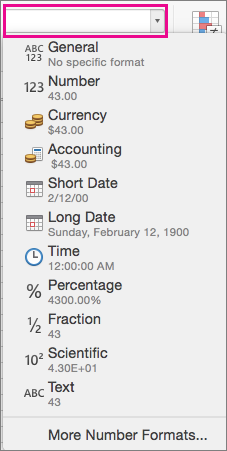
You can use number formats to change the appearance of numbers, including dates and times, without changing the actual number. The number format does not affect the cell value that Excel uses to perform calculations. The actual value is displayed in the formula bar.
Select a number format
-
Select the cells that you want to adjust.
-
On the Home tab, select a number format on the Number Format box. Data from a selected cell is shown in each possible format.
Display or hide the thousands separator
-
Select the cells that you want to adjust.
-
On the Home tab, click Comma Style

Note: Excel uses the Mac OS system separator for thousands. You can specify a different system separator by changing the regional settings in Mac OS X International system preferences.
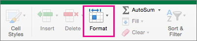
Change the display of negative numbers
You can format negative numbers by using minus signs, by enclosing them in parentheses, or by displaying them in a red font color either within opening and closing parentheses or without parentheses.
-
Select the cells that you want to adjust.
-
On the Home tab, click Format, and then click Format cells.
-
Do one of the following:
To display
Do this
Simple numbers
In the Category list, click Number.
Currency
In the Category list, click Currency.
-
In the Negative numbers box, select the display style that you want to use for negative numbers.
Control the display of digits after the decimal point in a number
The display format for a number is different from the actual number that is stored in a cell. For example, a number might be displayed as rounded off when there are too many digits after the decimal point for the number to display fully in a column. However, any calculations that include this number will use the actual number that is stored in the cell, not the rounded-off form that is displayed. To control how Excel displays digits after the decimal point, you can adjust the column width to accommodate the actual number of digits in the number, or you can specify how many of these digits are to be displayed for a number in a cell.
-
Select the cells that you want to adjust.
-
On the Home tab, click either Increase Decimal


See also
Create and apply a custom number format
Display numbers as postal codes, Social Security numbers, or phone numbers


