
Whether you need to forecast expenses for the next year or project the expected results for a series in a scientific experiment, you can use Microsoft Office Excel to automatically generate future values that are based on existing data or to automatically generate extrapolated values that are based on linear trend or growth trend calculations.
You can fill in a series of values that fit a simple linear trend or an exponential growth trend by using the fill handle or the Series command. To extend complex and nonlinear data, you can use worksheet functions or the regression analysis tool in the Analysis ToolPak Add-in.
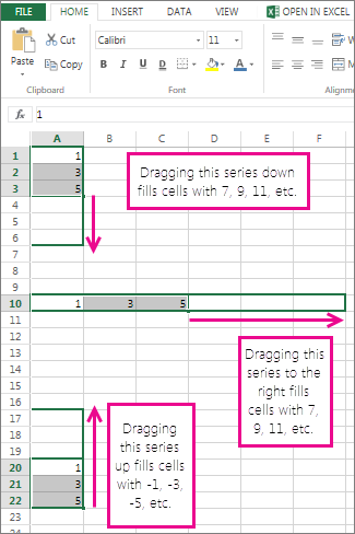
In a linear series, the step value, or the difference between the first and next value in the series, is added to the starting value and then added to each subsequent value.
|
Initial selection |
Extended linear series |
|---|---|
|
1, 2 |
3, 4, 5 |
|
1, 3 |
5, 7, 9 |
|
100, 95 |
90, 85 |
To fill in a series for a linear best-fit trend, do the following:
-
Select at least two cells that contain the starting values for the trend.
If you want to increase the accuracy of the trend series, select additional starting values.
-
Drag the fill handle in the direction that you want to fill with increasing values or decreasing values.
For example, if the selected starting values in cells C1:E1 are 3, 5, and 8, drag the fill handle to the right to fill with increasing trend values, or drag it to the left to fill with decreasing values.
Tip: To manually control how the series is created or to use the keyboard to fill in a series, click the Series command (Home tab, Editing group, Fill button).
In a growth series, the starting value is multiplied by the step value to get the next value in the series. The resulting product and each subsequent product are then multiplied by the step value.
|
Initial selection |
Extended growth series |
|---|---|
|
1, 2 |
4, 8, 16 |
|
1, 3 |
9, 27, 81 |
|
2, 3 |
4.5, 6.75, 10.125 |
To fill in a series for a growth trend, do the following:
-
Select at least two cells that contain the starting values for the trend.
If you want to increase the accuracy of the trend series, select additional starting values.
-
Hold down the right mouse button, drag the fill handle in the direction that you want to fill with increasing values or decreasing values, release the mouse button, and then click Growth Trend on the shortcut menu.
For example, if the selected starting values in cells C1:E1 are 3, 5, and 8, drag the fill handle to the right to fill with increasing trend values, or drag it to the left to fill with decreasing values.
Tip: To manually control how the series is created or to use the keyboard to fill in a series, click the Series command (Home tab, Editing group, Fill button).
When you click the Series command, you can manually control how a linear trend or growth trend is created and then use the keyboard to fill in the values.
-
In a linear series, the starting values are applied to the least-squares algorithm (y=mx+b) to generate the series.
-
In a growth series, the starting values are applied to the exponential curve algorithm (y=b*m^x) to generate the series.
In either case, the step value is ignored. The series that is created is equivalent to the values that are returned by the TREND function or GROWTH function.
To fill in the values manually, do the following:
-
Select the cell where you want to start the series. The cell must contain the first value in the series.
When you click the Series command, the resulting series replaces the original selected values. If you want to save the original values, copy them to a different row or column, and then create the series by selecting the copied values.
-
On the Home tab, in the Editing group, click Fill, and then click Series.
-
Do one of the following:
-
To fill the series down the worksheet, click Columns.
-
To fill the series across the worksheet, click Rows.
-
-
In the Step value box, enter the value that you want to increase the series by.
|
Series type |
Step value result |
|---|---|
|
Linear |
The step value is added to the first starting value and then added to each subsequent value. |
|
Growth |
The first starting value is multiplied by the step value. The resulting product and each subsequent product are then multiplied by the step value. |
-
Under Type, click Linear or Growth.
-
In the Stop value box, enter the value that you want to stop the series at.
Note: If there is more than one starting value in the series and you want Excel to generate the trend, select the Trend check box.
When you have existing data for which you want to forecast a trend, you can create a trendline in a chart. For example, if you have a chart in Excel that shows sales data for the first several months of the year, you can add a trendline to the chart that shows the general trend of sales (increasing or decreasing or flat) or that shows the projected trend for months ahead.
This procedure assumes that you already created a chart that is based on existing data. If you have not done so, see the topic Create a chart.
-
Click the chart.
-
Click the data series to which you want to add a trendline or moving average.
-
On the Layout tab, in the Analysis group, click Trendline, and then click the type of regression trendline or moving average that you want.
-
To set options and format the regression trendline or moving average, right-click the trendline, and then click Format Trendline on the shortcut menu.
-
Select the trendline options, lines, and effects that you want.
-
If you select Polynomial, enter in the Order box the highest power for the independent variable.
-
If you select Moving Average, enter in the Period box the number of periods to be used to calculate the moving average.
-
Notes:
-
The Based on series box lists all the data series in the chart that support trendlines. To add a trendline to another series, click the name in the box, and then select the options that you want.
-
If you add a moving average to an xy (scatter) chart, the moving average is based on the order of the x values plotted in the chart. To get the result that you want, you may need to sort the x values before you add a moving average.
Important: Beginning with Excel version 2005, Excel adjusted the way it calculates the R2 value for linear trendlines on charts where the trendline intercept is set to zero (0). This adjustment corrects calculations that yielded incorrect R2values and aligns the R2 calculation with the LINEST function. As a result, you may see different R2 values displayed on charts previously created in prior Excel versions. For more information, see Changes to internal calculations of linear trendlines in a chart.
When you need to perform more complicated regression analysis — including calculating and plotting residuals — you can use the regression analysis tool in the Analysis ToolPak Add-in. For more information, see Load the Analysis ToolPak.
In Excel for the web, you can project values in a series by using worksheet functions, or you can click and drag the fill handle to create a linear trend of numbers. But you can’t create a growth trend by using the fill handle.
Here’s how you use the fill handle to create a linear trend of numbers in Excel for the web:
-
Select at least two cells that contain the starting values for the trend.
If you want to increase the accuracy of the trend series, select additional starting values.
-
Drag the fill handle in the direction that you want to fill with increasing values or decreasing values.
Using the FORECAST function The FORECAST function calculates, or predicts, a future value by using existing values. The predicted value is a y-value for a given x-value. The known values are existing x-values and y-values, and the new value is predicted by using linear regression. You can use this function to predict future sales, inventory requirements, and consumer trends.
Using the TREND function or GROWTH function The TREND and GROWTH functions can extrapolate future y-values that extend a straight line or exponential curve that best describes the existing data. They can also return only the y-values based on known x-values for the best-fit line or curve. To plot a line or curve that describes existing data, use the existing x-values and y-values returned by the TREND or GROWTH function.
Using the LINEST function or LOGEST function You can use the LINEST or LOGEST function to calculate a straight line or exponential curve from existing data. The LINEST function and LOGEST function return various regression statistics, including the slope and intercept of the best-fit line.
The following table contains links to more information about these worksheet functions.
|
Function |
Description |
|---|---|
|
Project values |
|
|
Project values that fit a straight trend line |
|
|
Project values that fit an exponential curve |
|
|
Calculate a straight line from existing data |
|
|
Calculate an exponential curve from existing data |
Need more help?
You can always ask an expert in the Excel Tech Community or get support in Communities.


