
Use LOOKUP, one of the lookup and reference functions, when you need to look in a single row or column and find a value from the same position in a second row or column.
For example, let's say you know the part number for an auto part, but you don't know the price. You can use the LOOKUP function to return the price in cell H2 when you enter the auto part number in cell H1.
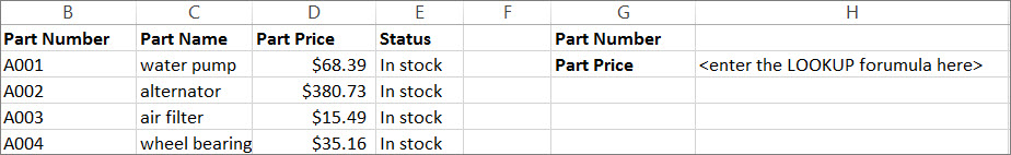
Use the LOOKUP function to search one row or one column. In the above example, we're searching prices in column D.
Tips: Consider one of the newer lookup functions, depending on which version you are using.
-
Use VLOOKUP to search one row or column, or to search multiple rows and columns (like a table). It's a much improved version of LOOKUP. Watch this video about how to use VLOOKUP.
-
If you are using Microsoft 365, use XLOOKUP - it's not only faster, it also lets you search in any direction (up, down, left, right).
There are two ways to use LOOKUP: Vector form and Array form
-
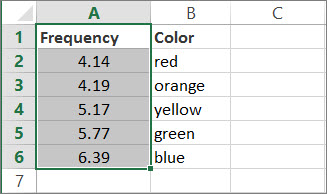
Vector form: Use this form of LOOKUP to search one row or one column for a value. Use the vector form when you want to specify the range that contains the values that you want to match. For example, if you want to search for a value in column A, down to row 6.
-
Array form: We strongly recommend using VLOOKUP or HLOOKUP instead of the array form. Watch this video about using VLOOKUP. The array form is provided for compatibility with other spreadsheet programs, but it's functionality is limited.
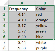
An array is a collection of values in rows and columns (like a table) that you want to search. For example, if you want to search columns A and B, down to row 6. LOOKUP will return the nearest match. To use the array form, your data must be sorted.
Vector form
The vector form of LOOKUP looks in a one-row or one-column range (known as a vector) for a value and returns a value from the same position in a second one-row or one-column range.
Syntax
LOOKUP(lookup_value, lookup_vector, [result_vector])
The LOOKUP function vector form syntax has the following arguments:
-
lookup_value Required. A value that LOOKUP searches for in the first vector. Lookup_value can be a number, text, a logical value, or a name or reference that refers to a value.
-
lookup_vector Required. A range that contains only one row or one column. The values in lookup_vector can be text, numbers, or logical values.
Important: The values in lookup_vector must be placed in ascending order: ..., -2, -1, 0, 1, 2, ..., A-Z, FALSE, TRUE; otherwise, LOOKUP might not return the correct value. Uppercase and lowercase text are equivalent.
-
result_vector Optional. A range that contains only one row or column. The result_vector argument must be the same size as lookup_vector. It has to be the same size.
Remarks
-
If the LOOKUP function can't find the lookup_value, the function matches the largest value in lookup_vector that is less than or equal to lookup_value.
-
If lookup_value is smaller than the smallest value in lookup_vector, LOOKUP returns the #N/A error value.
Vector examples
You can try out these examples in your own Excel worksheet to learn how the LOOKUP function works. In the first example, you're going to end up with a spreadsheet that looks similar to this one:
-
Copy the data in following table, and paste it into a new Excel worksheet.
Copy this data into column A
Copy this data into column B
Frequency
4.14
Color
red
4.19
orange
5.17
yellow
5.77
green
6.39
blue
-
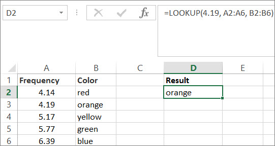
Next, copy the LOOKUP formulas from the following table into column D of your worksheet.
Copy this formula into the D column
Here's what this formula does
Here's the result you'll see
Formula
=LOOKUP(4.19, A2:A6, B2:B6)
Looks up 4.19 in column A, and returns the value from column B that is in the same row.
orange
=LOOKUP(5.75, A2:A6, B2:B6)
Looks up 5.75 in column A, matches the nearest smaller value (5.17), and returns the value from column B that is in the same row.
yellow
=LOOKUP(7.66, A2:A6, B2:B6)
Looks up 7.66 in column A, matches the nearest smaller value (6.39), and returns the value from column B that is in the same row.
blue
=LOOKUP(0, A2:A6, B2:B6)
Looks up 0 in column A, and returns an error because 0 is less than the smallest value (4.14) in column A.
#N/A
-
For these formulas to show results, you may need to select them in your Excel worksheet, press F2, and then press Enter. If you need to, adjust the column widths to see all the data.
Array form
Tip: We strongly recommend using VLOOKUP or HLOOKUP instead of the array form. See this video about VLOOKUP; it provides examples. The array form of LOOKUP is provided for compatibility with other spreadsheet programs, but its functionality is limited.
The array form of LOOKUP looks in the first row or column of an array for the specified value and returns a value from the same position in the last row or column of the array. Use this form of LOOKUP when the values that you want to match are in the first row or column of the array.
Syntax
LOOKUP(lookup_value, array)
The LOOKUP function array form syntax has these arguments:
-
lookup_value Required. A value that LOOKUP searches for in an array. The lookup_value argument can be a number, text, a logical value, or a name or reference that refers to a value.
-
If LOOKUP can't find the value of lookup_value, it uses the largest value in the array that is less than or equal to lookup_value.
-
If the value of lookup_value is smaller than the smallest value in the first row or column (depending on the array dimensions), LOOKUP returns the #N/A error value.
-
-
array Required. A range of cells that contains text, numbers, or logical values that you want to compare with lookup_value.
The array form of LOOKUP is very similar to the HLOOKUP and VLOOKUP functions. The difference is that HLOOKUP searches for the value of lookup_value in the first row, VLOOKUP searches in the first column, and LOOKUP searches according to the dimensions of array.
-
If array covers an area that is wider than it is tall (more columns than rows), LOOKUP searches for the value of lookup_value in the first row.
-
If an array is square or is taller than it is wide (more rows than columns), LOOKUP searches in the first column.
-
With the HLOOKUP and VLOOKUP functions, you can index down or across, but LOOKUP always selects the last value in the row or column.
Important: The values in array must be placed in ascending order: ..., -2, -1, 0, 1, 2, ..., A-Z, FALSE, TRUE; otherwise, LOOKUP might not return the correct value. Uppercase and lowercase text are equivalent.
-


