
Tip: Try using the new XLOOKUP and XMATCH functions, improved versions of the functions described in this article. These new functions work in any direction and return exact matches by default, making them easier and more convenient to use than their predecessors.
Suppose that you have a list of office location numbers, and you need to know which employees are in each office. The spreadsheet is huge, so you might think it is challenging task. It's actually quite easy to do with a lookup function.
The VLOOKUP and HLOOKUP functions, together with INDEX and MATCH, are some of the most useful functions in Excel.
Note: The Lookup Wizard feature is no longer available in Excel.
Here's an example of how to use VLOOKUP.
=VLOOKUP(B2,C2:E7,3,TRUE)
In this example, B2 is the first argument—an element of data that the function needs to work. For VLOOKUP, this first argument is the value that you want to find. This argument can be a cell reference, or a fixed value such as "smith" or 21,000. The second argument is the range of cells, C2-:E7, in which to search for the value you want to find. The third argument is the column in that range of cells that contains the value that you seek.
The fourth argument is optional. Enter either TRUE or FALSE. If you enter TRUE, or leave the argument blank, the function returns an approximate match of the value you specify in the first argument. If you enter FALSE, the function will match the value provide by the first argument. In other words, leaving the fourth argument blank—or entering TRUE—gives you more flexibility.
This example shows you how the function works. When you enter a value in cell B2 (the first argument), VLOOKUP searches the cells in the range C2:E7 (2nd argument) and returns the closest approximate match from the third column in the range, column E (3rd argument).
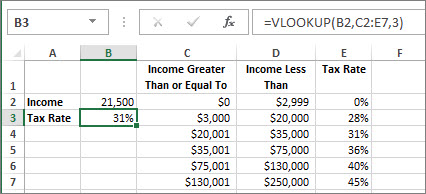
The fourth argument is empty, so the function returns an approximate match. If it didn't, you'd have to enter one of the values in columns C or D to get a result at all.
When you're comfortable with VLOOKUP, the HLOOKUP function is equally easy to use. You enter the same arguments, but it searches in rows instead of columns.
Using INDEX and MATCH instead of VLOOKUP
There are certain limitations with using VLOOKUP—the VLOOKUP function can only look up a value from left to right. This means that the column containing the value you look up should always be located to the left of the column containing the return value. Now if your spreadsheet isn't built this way, then do not use VLOOKUP. Use the combination of INDEX and MATCH functions instead.
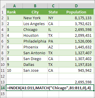
This example shows a small list where the value we want to search on, Chicago, isn't in the leftmost column. So, we can't use VLOOKUP. Instead, we'll use the MATCH function to find Chicago in the range B1:B11. It's found in row 4. Then, INDEX uses that value as the lookup argument, and finds the population for Chicago in the 4th column (column D). The formula used is shown in cell A14.
For more examples of using INDEX and MATCH instead of VLOOKUP, see the article https://www.mrexcel.com/excel-tips/excel-vlookup-index-match/ by Bill Jelen, Microsoft MVP.
Give it a try
If you want to experiment with lookup functions before you try them out with your own data, here's some sample data.
VLOOKUP Example at work
Copy the following data into a blank spreadsheet.
Tip: Before you paste the data into Excel, set the column widths for columns A through C to 250 pixels, and click Wrap Text (Home tab, Alignment group).
|
Density |
Viscosity |
Temperature |
|
0.457 |
3.55 |
500 |
|
0.525 |
3.25 |
400 |
|
0.606 |
2.93 |
300 |
|
0.675 |
2.75 |
250 |
|
0.746 |
2.57 |
200 |
|
0.835 |
2.38 |
150 |
|
0.946 |
2.17 |
100 |
|
1.09 |
1.95 |
50 |
|
1.29 |
1.71 |
0 |
|
Formula |
Description |
Result |
|
=VLOOKUP(1,A2:C10,2) |
Using an approximate match, searches for the value 1 in column A, finds the largest value less than or equal to 1 in column A which is 0.946, and then returns the value from column B in the same row. |
2.17 |
|
=VLOOKUP(1,A2:C10,3,TRUE) |
Using an approximate match, searches for the value 1 in column A, finds the largest value less than or equal to 1 in column A, which is 0.946, and then returns the value from column C in the same row. |
100 |
|
=VLOOKUP(0.7,A2:C10,3,FALSE) |
Using an exact match, searches for the value 0.7 in column A. Because there is no exact match in column A, an error is returned. |
#N/A |
|
=VLOOKUP(0.1,A2:C10,2,TRUE) |
Using an approximate match, searches for the value 0.1 in column A. Because 0.1 is less than the smallest value in column A, an error is returned. |
#N/A |
|
=VLOOKUP(2,A2:C10,2,TRUE) |
Using an approximate match, searches for the value 2 in column A, finds the largest value less than or equal to 2 in column A, which is 1.29, and then returns the value from column B in the same row. |
1.71 |
HLOOKUP Example
Copy all the cells in this table and paste it into cell A1 on a blank worksheet in Excel.
Tip: Before you paste the data into Excel, set the column widths for columns A through C to 250 pixels, and click Wrap Text (Home tab, Alignment group).
|
Axles |
Bearings |
Bolts |
|
4 |
4 |
9 |
|
5 |
7 |
10 |
|
6 |
8 |
11 |
|
Formula |
Description |
Result |
|
=HLOOKUP("Axles", A1:C4, 2, TRUE) |
Looks up "Axles" in row 1, and returns the value from row 2 that's in the same column (column A). |
4 |
|
=HLOOKUP("Bearings", A1:C4, 3, FALSE) |
Looks up "Bearings" in row 1, and returns the value from row 3 that's in the same column (column B). |
7 |
|
=HLOOKUP("B", A1:C4, 3, TRUE) |
Looks up "B" in row 1, and returns the value from row 3 that's in the same column. Because an exact match for "B" is not found, the largest value in row 1 that is less than "B" is used: "Axles," in column A. |
5 |
|
=HLOOKUP("Bolts", A1:C4, 4) |
Looks up "Bolts" in row 1, and returns the value from row 4 that's in the same column (column C). |
11 |
|
=HLOOKUP(3, {1,2,3;"a","b","c";"d","e","f"}, 2, TRUE) |
Looks up the number 3 in the three-row array constant, and returns the value from row 2 in the same (in this case, third) column. There are three rows of values in the array constant, each row separated by a semicolon (;). Because "c" is found in row 2 and in the same column as 3, "c" is returned. |
c |
INDEX and MATCH Examples
This last example employs the INDEX and MATCH functions together to return the earliest invoice number and its corresponding date for each of five cities. Because the date is returned as a number, we use the TEXT function to format it as a date. The INDEX function actually uses the result of the MATCH function as its argument. The combination of the INDEX and MATCH functions are used twice in each formula – first, to return the invoice number, and then to return the date.
Copy all the cells in this table and paste it into cell A1 on a blank worksheet in Excel.
Tip: Before you paste the data into Excel, set the column widths for columns A through D to 250 pixels, and click Wrap Text (Home tab, Alignment group).
|
Invoice |
City |
Invoice Date |
Earliest invoice by city, with date |
|
3115 |
Atlanta |
4/7/12 |
="Atlanta = "&INDEX($A$2:$C$33,MATCH("Atlanta",$B$2:$B$33,0),1)& ", Invoice date: " & TEXT(INDEX($A$2:$C$33,MATCH("Atlanta",$B$2:$B$33,0),3),"m/d/yy") |
|
3137 |
Atlanta |
4/9/12 |
="Austin = "&INDEX($A$2:$C$33,MATCH("Austin",$B$2:$B$33,0),1)& ", Invoice date: " & TEXT(INDEX($A$2:$C$33,MATCH("Austin",$B$2:$B$33,0),3),"m/d/yy") |
|
3154 |
Atlanta |
4/11/12 |
="Dallas = "&INDEX($A$2:$C$33,MATCH("Dallas",$B$2:$B$33,0),1)& ", Invoice date: " & TEXT(INDEX($A$2:$C$33,MATCH("Dallas",$B$2:$B$33,0),3),"m/d/yy") |
|
3191 |
Atlanta |
4/21/12 |
="New Orleans = "&INDEX($A$2:$C$33,MATCH("New Orleans",$B$2:$B$33,0),1)& ", Invoice date: " & TEXT(INDEX($A$2:$C$33,MATCH("New Orleans",$B$2:$B$33,0),3),"m/d/yy") |
|
3293 |
Atlanta |
4/25/12 |
="Tampa = "&INDEX($A$2:$C$33,MATCH("Tampa",$B$2:$B$33,0),1)& ", Invoice date: " & TEXT(INDEX($A$2:$C$33,MATCH("Tampa",$B$2:$B$33,0),3),"m/d/yy") |
|
3331 |
Atlanta |
4/27/12 |
|
|
3350 |
Atlanta |
4/28/12 |
|
|
3390 |
Atlanta |
5/1/12 |
|
|
3441 |
Atlanta |
5/2/12 |
|
|
3517 |
Atlanta |
5/8/12 |
|
|
3124 |
Austin |
4/9/12 |
|
|
3155 |
Austin |
4/11/12 |
|
|
3177 |
Austin |
4/19/12 |
|
|
3357 |
Austin |
4/28/12 |
|
|
3492 |
Austin |
5/6/12 |
|
|
3316 |
Dallas |
4/25/12 |
|
|
3346 |
Dallas |
4/28/12 |
|
|
3372 |
Dallas |
5/1/12 |
|
|
3414 |
Dallas |
5/1/12 |
|
|
3451 |
Dallas |
5/2/12 |
|
|
3467 |
Dallas |
5/2/12 |
|
|
3474 |
Dallas |
5/4/12 |
|
|
3490 |
Dallas |
5/5/12 |
|
|
3503 |
Dallas |
5/8/12 |
|
|
3151 |
New Orleans |
4/9/12 |
|
|
3438 |
New Orleans |
5/2/12 |
|
|
3471 |
New Orleans |
5/4/12 |
|
|
3160 |
Tampa |
4/18/12 |
|
|
3328 |
Tampa |
4/26/12 |
|
|
3368 |
Tampa |
4/29/12 |
|
|
3420 |
Tampa |
5/1/12 |
|
|
3501 |
Tampa |
5/6/12 |


