
This article was adapted from Microsoft Excel Data Analysis and Business Modeling by Wayne L. Winston.
-
Who uses Monte Carlo simulation?
-
What happens when you type =RAND() in a cell?
-
How can you simulate values of a discrete random variable?
-
How can you simulate values of a normal random variable?
-
How can a greeting card company determine how many cards to produce?
We would like to accurately estimate the probabilities of uncertain events. For example, what is the probability that a new product’s cash flows will have a positive net present value (NPV)? What is the risk factor of our investment portfolio? Monte Carlo simulation enables us to model situations that present uncertainty and then play them out on a computer thousands of times.
Note: The name Monte Carlo simulation comes from the computer simulations performed during the 1930s and 1940s to estimate the probability that the chain reaction needed for an atom bomb to detonate would work successfully. The physicists involved in this work were big fans of gambling, so they gave the simulations the code name Monte Carlo.
In the next five chapters, you will see examples of how you can use Excel to perform Monte Carlo simulations.
Many companies use Monte Carlo simulation as an important part of their decision-making process. Here are some examples.
-
General Motors, Proctor and Gamble, Pfizer, Bristol-Myers Squibb, and Eli Lilly use simulation to estimate both the average return and the risk factor of new products. At GM, this information is used by the CEO to determine which products come to market.
-
GM uses simulation for activities such as forecasting net income for the corporation, predicting structural and purchasing costs, and determining its susceptibility to different kinds of risk (such as interest rate changes and exchange rate fluctuations).
-
Lilly uses simulation to determine the optimal plant capacity for each drug.
-
Proctor and Gamble uses simulation to model and optimally hedge foreign exchange risk.
-
Sears uses simulation to determine how many units of each product line should be ordered from suppliers—for example, the number of pairs of Dockers trousers that should be ordered this year.
-
Oil and drug companies use simulation to value "real options," such as the value of an option to expand, contract, or postpone a project.
-
Financial planners use Monte Carlo simulation to determine optimal investment strategies for their clients’ retirement.
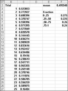
When you type the formula =RAND() in a cell, you get a number that is equally likely to assume any value between 0 and 1. Thus, around 25 percent of the time, you should get a number less than or equal to 0.25; around 10 percent of the time you should get a number that is at least 0.90, and so on. To demonstrate how the RAND function works, take a look at the file Randdemo.xlsx, shown in Figure 60-1.
Note: When you open the file Randdemo.xlsx, you will not see the same random numbers shown in Figure 60-1. The RAND function always automatically recalculates the numbers it generates when a worksheet is opened or when new information is entered into the worksheet.
First, copy from cell C3 to C4:C402 the formula =RAND(). Then you name the range C3:C402 Data. Then, in column F, you can track the average of the 400 random numbers (cell F2) and use the COUNTIF function to determine the fractions that are between 0 and 0.25, 0.25 and 0.50, 0.50 and 0.75, and 0.75 and 1. When you press the F9 key, the random numbers are recalculated. Notice that the average of the 400 numbers is always approximately 0.5, and that around 25 percent of the results are in intervals of 0.25. These results are consistent with the definition of a random number. Also note that the values generated by RAND in different cells are independent. For example, if the random number generated in cell C3 is a large number (for example, 0.99), it tells us nothing about the values of the other random numbers generated.
Suppose the demand for a calendar is governed by the following discrete random variable:
|
Demand |
Probability |
|
10,000 |
0.10 |
|
20,000 |
0.35 |
|
40,000 |
0.3 |
|
60,000 |
0.25 |
How can we have Excel play out, or simulate, this demand for calendars many times? The trick is to associate each possible value of the RAND function with a possible demand for calendars. The following assignment ensures that a demand of 10,000 will occur 10 percent of the time, and so on.
|
Demand |
Random number assigned |
|
10,000 |
Less than 0.10 |
|
20,000 |
Greater than or equal to 0.10, and less than 0.45 |
|
40,000 |
Greater than or equal to 0.45, and less than 0.75 |
|
60,000 |
Greater than or equal to 0.75 |
To demonstrate the simulation of demand, look at the file Discretesim.xlsx, shown in Figure 60-2 on the next page.
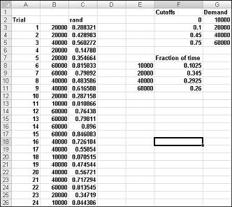
The key to our simulation is to use a random number to initiate a lookup from the table range F2:G5 (named lookup). Random numbers greater than or equal to 0 and less than 0.10 will yield a demand of 10,000; random numbers greater than or equal to 0.10 and less than 0.45 will yield a demand of 20,000; random numbers greater than or equal to 0.45 and less than 0.75 will yield a demand of 40,000; and random numbers greater than or equal to 0.75 will yield a demand of 60,000. You generate 400 random numbers by copying from C3 to C4:C402 the formula RAND(). You then generate 400 trials, or iterations, of calendar demand by copying from B3 to B4:B402 the formula VLOOKUP(C3,lookup,2). This formula ensures that any random number less than 0.10 generates a demand of 10,000, any random number between 0.10 and 0.45 generates a demand of 20,000, and so on. In the cell range F8:F11, use the COUNTIF function to determine the fraction of our 400 iterations yielding each demand. When we press F9 to recalculate the random numbers, the simulated probabilities are close to our assumed demand probabilities.
If you type in any cell the formula NORMINV(rand(),mu,sigma), you will generate a simulated value of a normal random variable having a mean mu and standard deviation sigma. This procedure is illustrated in the file Normalsim.xlsx, shown in Figure 60-3.
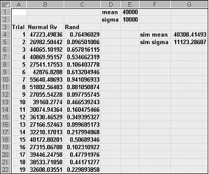
Let’s suppose we want to simulate 400 trials, or iterations, for a normal random variable with a mean of 40,000 and a standard deviation of 10,000. (You can type these values in cells E1 and E2, and name these cells mean and sigma, respectively.) Copying the formula =RAND() from C4 to C5:C403 generates 400 different random numbers. Copying from B4 to B5:B403 the formula NORMINV(C4,mean,sigma) generates 400 different trial values from a normal random variable with a mean of 40,000 and a standard deviation of 10,000. When we press the F9 key to recalculate the random numbers, the mean remains close to 40,000 and the standard deviation close to 10,000.
Essentially, for a random number x, the formula NORMINV(p,mu,sigma) generates the pth percentile of a normal random variable with a mean mu and a standard deviation sigma. For example, the random number 0.77 in cell C4 (see Figure 60-3) generates in cell B4 approximately the 77th percentile of a normal random variable with a mean of 40,000 and a standard deviation of 10,000.
In this section, you will see how Monte Carlo simulation can be used as a decision-making tool. Suppose that the demand for a Valentine’s Day card is governed by the following discrete random variable:
|
Demand |
Probability |
|
10,000 |
0.10 |
|
20,000 |
0.35 |
|
40,000 |
0.3 |
|
60,000 |
0.25 |
The greeting card sells for $4.00, and the variable cost of producing each card is $1.50. Leftover cards must be disposed of at a cost of $0.20 per card. How many cards should be printed?
Basically, we simulate each possible production quantity (10,000, 20,000, 40,000, or 60,000) many times (for example, 1000 iterations). Then we determine which order quantity yields the maximum average profit over the 1000 iterations. You can find the data for this section in the file Valentine.xlsx, shown in Figure 60-4. You assign the range names in cells B1:B11 to cells C1:C11. The cell range G3:H6 is assigned the name lookup. Our sales price and cost parameters are entered in cells C4:C6.
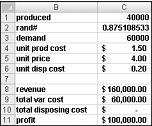
You can enter a trial production quantity (40,000 in this example) in cell C1. Next, create a random number in cell C2 with the formula =RAND(). As previously described, you simulate demand for the card in cell C3 with the formula VLOOKUP(rand,lookup,2). (In the VLOOKUP formula, rand is the cell name assigned to cell C3, not the RAND function.)
The number of units sold is the smaller of our production quantity and demand. In cell C8, you compute our revenue with the formula MIN(produced,demand)*unit_price. In cell C9, you compute total production cost with the formula produced*unit_prod_cost.
If we produce more cards than are in demand, the number of units left over equals production minus demand; otherwise no units are left over. We compute our disposal cost in cell C10 with the formula unit_disp_cost*IF(produced>demand,produced–demand,0). Finally, in cell C11, we compute our profit as revenue– total_var_cost-total_disposing_cost.
We would like an efficient way to press F9 many times (for example, 1000) for each production quantity and tally our expected profit for each quantity. This situation is one in which a two-way data table comes to our rescue. (See Chapter 15, "Sensitivity Analysis with Data Tables," for details about data tables.) The data table used in this example is shown in Figure 60-5.
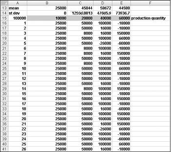
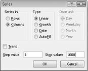
In the cell range A16:A1015, enter the numbers 1–1000 (corresponding to our 1000 trials). One easy way to create these values is to start by entering 1 in cell A16. Select the cell, and then on the Home tab in the Editing group, click Fill, and select Series to display the Series dialog box. In the Series dialog box, shown in Figure 60-6, enter a Step Value of 1 and a Stop Value of 1000. In the Series In area, select the Columns option, and then click OK. The numbers 1–1000 will be entered in column A starting in cell A16.
Next we enter our possible production quantities (10,000, 20,000, 40,000, 60,000) in cells B15:E15. We want to calculate profit for each trial number (1 through 1000) and each production quantity. We refer to the formula for profit (calculated in cell C11) in the upper-left cell of our data table (A15) by entering =C11.
We are now ready to trick Excel into simulating 1000 iterations of demand for each production quantity. Select the table range (A15:E1014), and then in the Data Tools group on the Data tab, click What If Analysis, and then select Data Table. To set up a two-way data table, choose our production quantity (cell C1) as the Row Input Cell and select any blank cell (we chose cell I14) as the Column Input Cell. After clicking OK, Excel simulates 1000 demand values for each order quantity.
To understand why this works, consider the values placed by the data table in the cell range C16:C1015. For each of these cells, Excel will use a value of 20,000 in cell C1. In C16, the column input cell value of 1 is placed in a blank cell and the random number in cell C2 recalculates. The corresponding profit is then recorded in cell C16. Then the column cell input value of 2 is placed in a blank cell, and the random number in C2 again recalculates. The corresponding profit is entered in cell C17.
By copying from cell B13 to C13:E13 the formula AVERAGE(B16:B1015), we compute average simulated profit for each production quantity. By copying from cell B14 to C14:E14 the formula STDEV(B16:B1015), we compute the standard deviation of our simulated profits for each order quantity. Each time we press F9, 1000 iterations of demand are simulated for each order quantity. Producing 40,000 cards always yields the largest expected profit. Therefore, it appears that producing 40,000 cards is the proper decision.
The Impact of Risk on Our Decision If we produced 20,000 instead of 40,000 cards, our expected profit drops approximately 22 percent, but our risk (as measured by the standard deviation of profit) drops almost 73 percent. Therefore, if we are extremely averse to risk, producing 20,000 cards might be the right decision. Incidentally, producing 10,000 cards always has a standard deviation of 0 cards because if we produce 10,000 cards, we will always sell all of them without any leftovers.
Note: In this workbook, the Calculation option is set to Automatic Except For Tables. (Use the Calculation command in the Calculation group on the Formulas tab.) This setting ensures that our data table will not recalculate unless we press F9, which is a good idea because a large data table will slow down your work if it recalculates every time you type something into your worksheet. Note that in this example, whenever you press F9, the mean profit will change. This happens because each time you press F9, a different sequence of 1000 random numbers is used to generate demands for each order quantity.
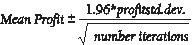
Confidence Interval for Mean Profit A natural question to ask in this situation is, into what interval are we 95 percent sure the true mean profit will fall? This interval is called the 95 percent confidence interval for mean profit. A 95 percent confidence interval for the mean of any simulation output is computed by the following formula:
In cell J11, you compute the lower limit for the 95 percent confidence interval on mean profit when 40,000 calendars are produced with the formula D13–1.96*D14/SQRT(1000). In cell J12, you compute the upper limit for our 95 percent confidence interval with the formula D13+1.96*D14/SQRT(1000). These calculations are shown in Figure 60-7.
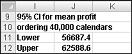
We are 95 percent sure that our mean profit when 40,000 calendars are ordered is between $56,687 and $62,589.
-
A GMC dealer believes that demand for 2005 Envoys will be normally distributed with a mean of 200 and standard deviation of 30. His cost of receiving an Envoy is $25,000, and he sells an Envoy for $40,000. Half of all the Envoys not sold at full price can be sold for $30,000. He is considering ordering 200, 220, 240, 260, 280, or 300 Envoys. How many should he order?
-
A small supermarket is trying to determine how many copies of People magazine they should order each week. They believe their demand for People is governed by the following discrete random variable:
Demand
Probability
15
0.10
20
0.20
25
0.30
30
0.25
35
0.15
-
The supermarket pays $1.00 for each copy of People and sells it for $1.95. Each unsold copy can be returned for $0.50. How many copies of People should the store order?
Need more help?
You can always ask an expert in the Excel Tech Community or get support in Communities.


