#VALUE is Excel's way of saying, "There's something wrong with the way your formula is typed. Or, there's something wrong with the cells you are referencing." The error is very general, and it can be hard to find the exact cause of it. The information on this page shows common problems and solutions for the error.
Use the drop-down below or jump to one of the other areas:
Fix the error for a specific function
See more information at Correct the #VALUE! error in AVERAGE or SUM functions
See more information at Correct the #VALUE! error in the CONCATENATE function
See more information at Correct the #VALUE! error in the COUNTIF/COUNTIFS function
See more information at Correct the #VALUE! error in the DATEVALUE function
See more information at Correct the #VALUE! error in the DAYS function
See more information at Correct the #VALUE! error in the FIND/FINDB and SEARCH/SEARCHB functions
See more information at Correct the #VALUE! error in the IF function
See more information at Correct the #VALUE! error in the INDEX and MATCH functions
See more information at Correct the #VALUE! error in the FIND/FINDB and SEARCH/SEARCHB functions
See more information at Correct the #VALUE! error in AVERAGE or SUM functions
See more information at Correct the #VALUE! error in the SUMIF/SUMIFS function
See more information at Correct the #VALUE! error in the SUMPRODUCT function
See more information at Correct the #VALUE! error in the TIMEVALUE function
See more information at Correct the #VALUE! error in the TRANSPOSE function
See more information at Correct the #VALUE! error in the VLOOKUP function
Don’t see your function in this list? Try the other solutions listed below.
Problems with subtraction
If you're new to Excel, you might be typing a formula for subtraction incorrectly. Here are two ways to do it:
Subtract a cell reference from another
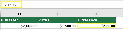
Type two values in two separate cells. In a third cell, subtract one cell reference from the other. In this example, cell D2 has the budgeted amount, and cell E2 has the actual amount. F2 has the formula =D2-E2.
Or, use SUM with positive and negative numbers
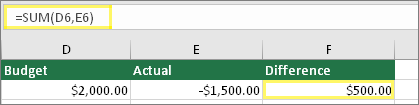
Type a positive value in one cell, and a negative value in another. In a third cell, use the SUM function to add the two cells together. In this example, cell D6 has the budgeted amount, and cell E6 has the actual amount as a negative number. F6 has the formula =SUM(D6,E6).
If you're using Windows, you might get the #VALUE! error when doing even the most basic subtraction formula. The following might solve your problem:
-
First do a quick test. In a new workbook, type a 2 in cell A1. Type a 4 in cell B1. Then in C1 type this formula =B1-A1. If you get the #VALUE! error, go to the next step. If you don't get the error, try other solutions on this page.
-
In Windows, open your Region control panel.
-
Windows 10: Select Start, type Region, and then select the Region control panel.
-
Windows 8: At the Start screen, type Region, select Settings, and then select Region.
-
Windows 7: Select Start, type Region, and then select Region and language.
-
-
On the Formats tab, select Additional settings.
-
Look for the List separator. If the List separator is set to the minus sign, change it to something else. For example, a comma is a common list separator. The semicolon is also common. However, another list separator might be more appropriate for your particular region.
-
Select OK.
-
Open your workbook. If a cell contains a #VALUE! error, double-click to edit it.
-
If there are commas where there should be minus signs for subtraction, change them to minus signs.
-
Press ENTER.
-
Repeat this process for other cells that have the error.
Subtract a cell reference from another
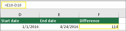
Type two dates in two separate cells. In a third cell, subtract one cell reference from the other. In this example, cell D10 has the start date, and cell E10 has the End date. F10 has the formula =E10-D10.
Or, use the DATEDIF function
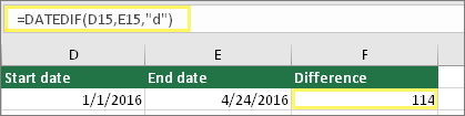
Type two dates in two separate cells. In a third cell, use the DATEDIF function to find the difference in dates. For more information on the DATEDIF function, see Calculate the difference between two dates.
Make your date column wider. If your date is aligned to the right, then it's a date. But if it's aligned to the left, this means the date isn't really a date. It's text. And Excel won't recognize text as a date. Here are some solutions that can help this problem.
Check for leading spaces
-
Double-click a date that is being used in a subtraction formula.
-
Put your cursor at the beginning and see if you can select one or more spaces. Here's what a selected space looks like at the beginning of a cell:

If your cell has this problem, proceed to the next step. If you don't see one or more spaces, go to the next section on checking your computer's date settings.
-
Select the column that contains the date by selecting its column header.
-
Select Data > Text to Columns.
-
Select Next twice.
-
On Step 3 of 3 of the wizard, under Column data format, select Date.
-
Choose a date format, and then select Finish.
-
Repeat this process for other columns to ensure they don't contain leading spaces before dates.
Check your computer's date settings
Excel uses your computer's date system. If a cell's date isn't entered using the same date system, Excel won't recognize it as a true date.
For example, let's say that your computer displays dates as mm/dd/yyyy. If you typed a date like that in a cell, Excel would recognize it as a date and you'd be able to use it in a subtraction formula. However, if you typed a date like dd/mm/yy, Excel wouldn't recognize that as a date. Instead, it would treat it as text.
There are two solutions to this problem: You could change the date system that your computer uses to match the date system you want to type in Excel. Or, in Excel you could create a new column and use the DATE function to create a true date based on the date stored as text. Here's how to do that assuming your computers date system is mm/dd/yyy and your text date is 31/12/2017 in cell A1:
-
Create a formula like this: =DATE(RIGHT(A1,4),MID(A1,4,2),LEFT(A1,2))
-
The result would be 12/31/2017.
-
If you want the format to appear like dd/mm/yy, press CTRL+1 (or
-
Choose a different locale that uses the dd/mm/yy format, for example, English (United Kingdom). When you're done applying the format, the result is 31/12/2017 and it is a true date, not a text date.

Problems with spaces and text
Often #VALUE! occurs because your formula refers to other cells that contain spaces, or even trickier: hidden spaces. These spaces can make a cell look blank, when in fact they are not blank.
1. Select referenced cells
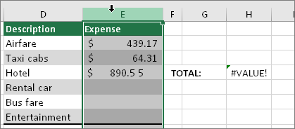
Find cells that your formula is referencing and select them. In many cases removing spaces for an entire column is a good practice because you can replace more than one space at a time. In this example, selecting the E selects the entire column.
2. Find and replace

On the Home tab, select Find & Select > Replace.
3. Replace spaces with nothing
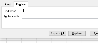
In the Find what box, type a single space. Then, in the Replace with box, delete anything that might be there.
4. Replace or Replace all
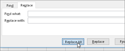
If you are confident that all spaces in the column should be removed, select Replace All. If you'd like to step through and replace spaces with nothing on an individual basis, you can select Find next first, and then select Replace when you're confident the space isn't needed. When you're done, the #VALUE! error might be resolved. If not, go to the next step.
5. Turn on the filter
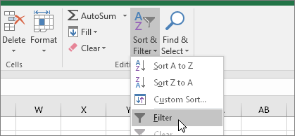
Sometimes hidden characters other than spaces can make a cell appear blank, when it's not really blank. Single apostrophes within a cell can do this. To get rid of these characters in a column, turn on the filter by going to Home > Sort & Filter > Filter.
6. Set the filter

Click the filter arrow 
7. Select any unnamed checkboxes
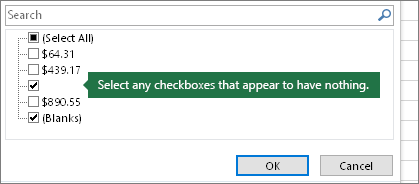
Select any check boxes that don't have anything next to them, like this one.
8. Select blank cells, and delete

When Excel brings back the blank cells, select them. Then press the Delete key. This clears any hidden characters in the cells.
9. Clear the filter
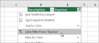
Select the filter arrow
10. Result
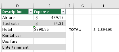
If spaces were the culprit of your #VALUE! error then hopefully your error has been replaced by the formula result, as shown here in our example. If not, repeat this process for other cells that your formula refers to. Or, try other solutions on this page.
Note: In this example, notice that cell E4 has a green triangle and the number is aligned to the left. This means the number is stored as text. This could cause more problems later. If you see this problem, we recommend converting numbers stored as text to numbers.
Text or special characters within a cell can cause the #VALUE! error. But sometimes it's hard to see which cells have these problems. Solution: Use the ISTEXT function to inspect cells. Note that ISTEXT doesn't resolve the error, it simply finds cells that might be causing the error.
Example with #VALUE!
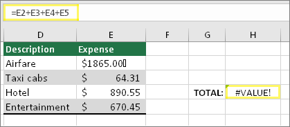
Here’s an example of a formula that has a #VALUE! error. This is likely due to cell E2. A special character appears as a small box after "00." Or as the next picture shows, you could use the ISTEXT function in a separate column to check for text.
Same example, with ISTEXT
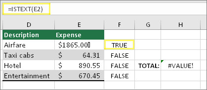
Here the ISTEXT function was added in column F. All cells are fine except the one with the value of TRUE. This means cell E2 has text. To resolve this, you could delete the cell's contents and retype the value of 1865.00. Or you could also use the CLEAN function to clean out characters, or use the REPLACE function to replace special characters with other values.
After using CLEAN or REPLACE, you'll want to copy the result, and use Home > Paste > Paste Special > Values. You might also have to convert numbers stored as text to numbers.
Formulas with math operations like + and * might not be able to calculate cells that contain text or spaces. In this case, try using a function instead. Functions often ignore text values and calculate everything as numbers, eliminating the #VALUE! error. For example, instead of =A2+B2+C2, type =SUM(A2:C2). Or, instead of =A2*B2, type =PRODUCT(A2,B2).
Other solutions to try
Select the error

First select the cell with the #VALUE! error.
Click Formulas > Evaluate Formula
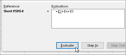
Select Formulas > Evaluate Formula > Evaluate. Excel steps through the parts of the formula individually. In this case the formula =E2+E3+E4+E5 breaks because of a hidden space in cell E2. You can't see the space by looking at cell E2. However, you can see it here. It shows as " ".
Sometimes you just want to replace the #VALUE! error with something else like your own text, a zero or a blank cell. In this case you can add the IFERROR function to your formula. IFERROR checks to see if there’s an error, and if so, replaces it with another value of your choice. If there isn’t an error, your original formula is calculated.
Warning: IFERROR hides all errors, not just the #VALUE! error. Hiding errors isn't recommended because an error is often a sign that something needs to be fixed, not hidden. We don't recommend using this function unless you're absolutely certain your formula works the way that you want.
Cell with #VALUE!
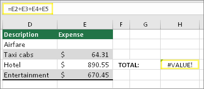
Here’s an example of a formula that has a #VALUE! error due to a hidden space in cell E2.
Error hidden by IFERROR
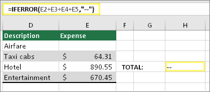
And here’s the same formula with IFERROR added to the formula. You can read the formula as: "Calculate the formula, but if there's any kind of error, replace it with two dashes." Note that you could also use "" to display nothing instead of two dashes. Or you could substitute your own text, such as: "Total Error".
Unfortunately, you can see that IFERROR doesn’t actually resolve the error, it simply hides it. So be certain that hiding the error is better than fixing it.
Your data connection could have become unavailable at some point. To fix this, restore the data connection, or consider importing the data if possible. If you don't have access to the connection, ask the creator of the workbook to make a new file for you. The new file ideally would have only values, and no connections. They can do this by copying all the cells and pasting only as values. To paste as only values, they can select Home > Paste > Paste Special > Values. This eliminates all formulas and connections, and therefore would also remove any #VALUE! errors.
If you’re not sure what to do at this point, you can search for similar questions in the Excel Community Forum, or post one of your own.