
The GETPIVOTDATA function returns visible data from a PivotTable.
In this example, =GETPIVOTDATA("Sales",A3) returns the total sales amount from a PivotTable:

Syntax
GETPIVOTDATA(data_field, pivot_table, [field1, item1, field2, item2], ...)
The GETPIVOTDATA function syntax has the following arguments:
|
Argument |
Description |
|---|---|
|
data_field Required |
The name of the PivotTable field that contains the data that you want to retrieve. This needs to be in quotes. |
|
pivot_table Required |
A reference to any cell, range of cells, or named range of cells in a PivotTable. This information is used to determine which PivotTable contains the data that you want to retrieve. |
|
field1, item1, field2, item2... Optional |
1 to 126 pairs of field names and item names that describe the data that you want to retrieve. The pairs can be in any order. Field names and names for items other than dates and numbers need to be enclosed in quotation marks. For OLAP PivotTables, items can contain the source name of the dimension and also the source name of the item. A field and item pair for an OLAP PivotTable might look like this: "[Product]","[Product].[All Products].[Foods].[Baked Goods]" |
Notes:
-
You can quickly enter a simple GETPIVOTDATA formula by typing = (the equal sign) in the cell you want to return the value to and then clicking the cell in the PivotTable that contains the data you want to return.
-
You can turn this feature off by selecting any cell within an existing PivotTable, then go to the PivotTable Analyze tab > PivotTable > Options > Uncheck the Generate GetPivotData option.
-
Calculated fields or items and custom calculations can be included in GETPIVOTDATA calculations.
-
If the pivot_table argument is a range that includes two or more PivotTables, data will be retrieved from whichever PivotTable was created most recently.
-
If the field and item arguments describe a single cell, then the value of that cell is returned regardless of whether it is a string, number, error, or blank cell.
-
If an item contains a date, the value must be expressed as a serial number or populated by using the DATE function so that the value will be retained if the worksheet is opened in a different locale. For example, an item referring to the date March 5, 1999 could be entered as 36224 or DATE(1999,3,5). Times can be entered as decimal values or by using the TIME function.
-
If the pivot_table argument is not a range in which a PivotTable is found, GETPIVOTDATA returns #REF!.
-
If the arguments do not describe a visible field, or if they include a report filter in which the filtered data is not displayed, GETPIVOTDATA returns the #REF! error value.
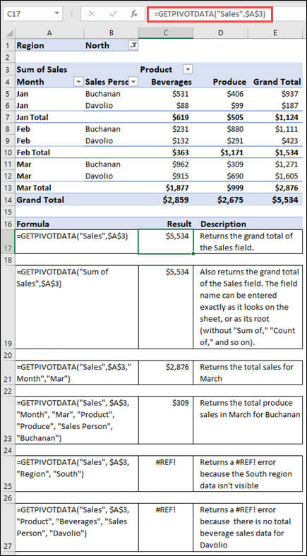
Examples
The formulas in the example below show various methods for getting data from a PivotTable.
Need more help?
You can always ask an expert in the Excel Tech Community or get support in Communities.
See Also


