
Let's say that your spreadsheet formulas have errors that you anticipate and don't need to correct, but you want to improve the display of your results. There are several ways to hide error values and error indicators in cells.
There are many reasons why formulas can return errors. For example, division by 0 is not allowed, and if you enter the formula =1/0, Excel returns #DIV/0. Error values include #DIV/0!, #N/A, #NAME?, #NULL!, #NUM!, #REF!, and #VALUE!.
Convert an error to zero and use a format to hide the value
You can hide error values by converting them to a number such as 0, and then applying a conditional format that hides the value.
Create an example error
-
Open a blank workbook, or create a new worksheet.
-
Enter 3 in cell B1, enter 0 in cell C1, and in cell A1, enter the formula =B1/C1.
The #DIV/0! error appears in cell A1. -
Select A1, and press F2 to edit the formula.
-
After the equal sign (=), type IFERROR followed by an opening parenthesis.
IFERROR( -
Move the cursor to the end of the formula.
-
Type ,0) – that is, a comma followed by a zero and a closing parenthesis.
The formula =B1/C1 becomes =IFERROR(B1/C1,0). -
Press Enter to complete the formula.
The contents of the cell should now display 0 instead of the #DIV! error.
Apply the conditional format
-
Select the cell that contains the error, and on the Home tab, click Conditional Formatting.
-
Click New Rule.
-
In the New Formatting Rule dialog box, click Format only cells that contain.
-
Under Format only cells with, make sure Cell Value appears in the first list box, equal to appears in the second list box, and then type 0 in the text box to the right.
-
Click the Format button.
-
Click the Number tab and then, under Category, click Custom.
-
In the Type box, enter ;;; (three semicolons), and then click OK. Click OK again.
The 0 in the cell disappears. This happens because the ;;; custom format causes any numbers in a cell to not be displayed. However, the actual value (0) remains in the cell.
Use the following procedure to format cells that contain errors so that the text in those cells is displayed in a white font. This makes the error text in these cells virtually invisible.
-
Select the range of cells that contain the error value.
-
On the Home tab, select the arrow next to Conditional Formatting and then click Manage Rules.
The Conditional Formatting Rules Manager dialog box appears. -
Click New Rule.
The New Formatting Rule dialog box appears. -
Under Select a Rule Type, click Format only cells that contain.
-
Under Edit the Rule Description, in the Format only cells with list, select Errors.
-
Click Format, and then click the Font tab.
-
Click the arrow to open the Color list, and under Theme Colors, select the white color.
There may be times when you do not want error vales to appear in cells, and would prefer that a text string such as “#N/A,” a dash, or the string “NA” appears instead. To do this, you can use the IFERROR and NA functions, as the following example shows.
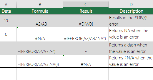
Function details
IFERROR Use this function to determine if a cell contains an error or if the results of a formula will return an error.
NA Use this function to return the string #N/A in a cell. The syntax is =NA().
-
Click the PivotTable report.
-
On the PivotTable Analyze tab, in the PivotTable group, click the arrow next to Options, and then click Options.
-
Click the Layout & Format tab, and then do one or more of the following:
-
Change error display Select the For error values show check box under Format. In the box, type the value that you want to display instead of errors. To display errors as blank cells, delete any characters in the box.
-
Change empty cell display Select the For empty cells show check box. In the box, type the value that you want to display in empty cells. To display blank cells, delete any characters in the box. To display zeros, clear the check box.
-
If a cell contains a formula that results in an error, a triangle (an error indicator) appears in the top-left corner of the cell. You can prevent these indicators from being displayed by using the following procedure.

Cell with a formula problem
-
On the File tab, select Options and choose Formulas.
-
Under Error Checking, clear the Enable background error checking check box.


