Sign in with Microsoft
Sign in or create an account.
Hello,
Select a different account.
You have multiple accounts
Choose the account you want to sign in with.

Important: Some of the content in this topic may not be applicable to some languages.

You can quickly filter data based on visual criteria, such as font color, cell color, or icon sets. And you can filter whether you have formatted cells, applied cell styles, or used conditional formatting.

  1. In a range of cells or a table column, click a cell that contains the cell color, font color, or icon that you want to filter by.

  2. On the Data tab, click Filter.
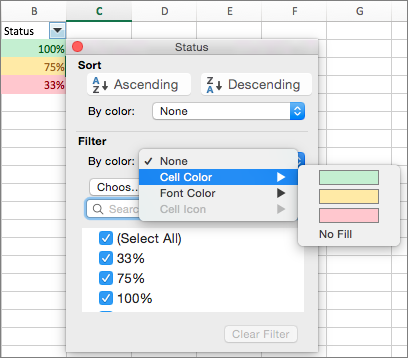
    On the Data tab, select Filter

  3. Click the arrow AutoFilter arrow in the column that contains the content that you want to filter.

  4. Under Filter, in the By color pop-up menu, select Cell Color, Font Color, or Cell Icon, and then click the criteria.

    Example of filtering by cell color

See Also

Use data bars, color scales, and icon sets to highlight data

Filter a list of data

Apply, create, or remove a cell style

Need more help?

Want more options?

Explore subscription benefits, browse training courses, learn how to secure your device, and more.

Communities help you ask and answer questions, give feedback, and hear from experts with rich knowledge.

Was this information helpful?

What affected your experience?
By pressing submit, your feedback will be used to improve Microsoft products and services. Your IT admin will be able to collect this data. Privacy Statement.

Thank you for your feedback!

×