
Filter data in a range or table
Use AutoFilter or built-in comparison operators like "greater than" and “top 10” in Excel to show the data you want and hide the rest. Once you filter data in a range of cells or table, you can either reapply a filter to get up-to-date results, or clear a filter to redisplay all of the data.
Use filters to temporarily hide some of the data in a table, so you can focus on the data you want to see.

Filter a range of data
-
Select any cell within the range.
-
Select Data > Filter.

-
Select the column header arrow

-
Select Text Filters or Number Filters, and then select a comparison, like Between.

-
Enter the filter criteria and select OK.

Filter data in a table
When you put your data in a table, filter controls are automatically added to the table headers.

-
Select the column header arrow

-
Uncheck (Select All) and select the boxes you want to show.

-
Select OK.
The column header arrow

Related Topics
Excel Training: Filter data in a table
Guidelines and examples for sorting and filtering data by color
Filtered data displays only the rows that meet criteria that you specify and hides rows that you do not want displayed. After you filter data, you can copy, find, edit, format, chart, and print the subset of filtered data without rearranging or moving it.
You can also filter by more than one column. Filters are additive, which means that each additional filter is based on the current filter and further reduces the subset of data.
Note: When you use the Find dialog box to search filtered data, only the data that is displayed is searched; data that is not displayed is not searched. To search all the data, clear all filters.
The two types of filters
Using AutoFilter, you can create two types of filters: by a list value or by criteria. Each of these filter types is mutually exclusive for each range of cells or column table. For example, you can filter by a list of numbers, or a criteria, but not by both; you can filter by icon or by a custom filter, but not by both.
Reapplying a filter
To determine if a filter is applied, note the icon in the column heading:
-
A drop-down arrow
When you hover over the heading of a column with filtering enabled but not applied, a screen tip displays "(Showing All)".
-
A Filter button
When you hover over the heading of a filtered column, a screen tip displays the filter applied to that column, such as "Equals a red cell color" or "Larger than 150".
When you reapply a filter, different results appear for the following reasons:
-
Data has been added, modified, or deleted to the range of cells or table column.
-
Values returned by a formula have changed and the worksheet has been recalculated.
Do not mix data types
For best results, do not mix data types, such as text and number, or number and date in the same column, because only one type of filter command is available for each column. If there is a mix of data types, the command that is displayed is the data type that occurs the most. For example, if the column contains three values stored as number and four as text, the Text Filters command is displayed .
Filter data in a table
When you put your data in a table, filtering controls are added to the table headers automatically.
-
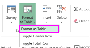
Select the data you want to filter. On the Home tab, select Format as Table, and then pick Format as Table.
-
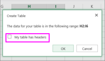
In the Create Table dialog box, you can choose whether your table has headers.
-
Select My table has headers to turn the top row of your data into table headers. The data in this row won't be filtered.
-
Don't select the check box if you want Excel for the web to add placeholder headers (that you can rename) above your table data.
-
-
Select OK.
-
To apply a filter, click the arrow in the column header, and pick a filter option.
Filter a range of data
If you don't want to format your data as a table, you can also apply filters to a range of data.
-
Select the data you want to filter. For best results, the columns should have headings.
-
On the Data tab, choose Filter.
Filtering options for tables or ranges
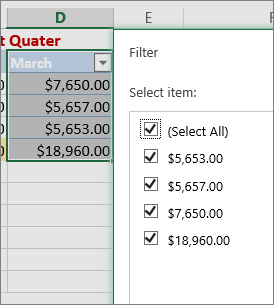
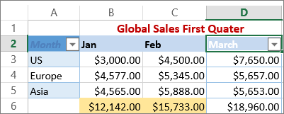
You can either apply a general Filter option or a custom filter specific to the data type. For example, when filtering numbers, you’ll see Number Filters, for dates you'll see Date Filters, and for text you'll see Text Filters. The general filter option lets you select the data you want to see from a list of existing data like this:
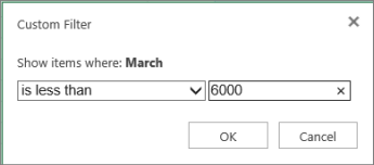
Number Filters lets you apply a custom filter:
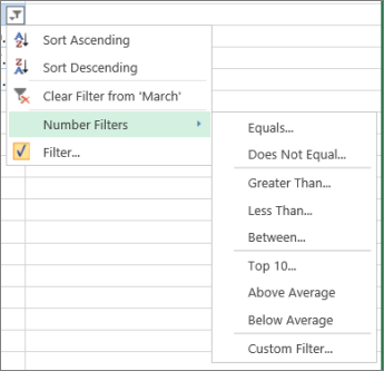
In this example, if you want to see the regions that had sales below $6,000 in March, you can apply a custom filter:
Here’s how:
-
Select the filter arrow next to March > Number Filters > Less Than and enter 6000.
-
Click OK.
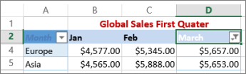
Excel for the web applies the filter and shows only the regions with sales below $6000.
You can apply custom Date Filters and Text Filters in a similar manner.
To clear a filter from a column
-
Select the Filter
To remove all the filters from a table or range
-
Select any cell inside your table or range and, on the Data tab, select the Filter button.
This will remove the filters from all the columns in your table or range and show all your data.
-
Click a cell in the range or table that you want to filter.
-
On the Data tab, select Filter.

-
Select the arrow

-
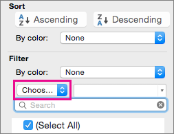
Under Filter, select Choose One, and then enter your filter criteria.
Notes:
-
You can apply filters to only one range of cells on a sheet at a time.
-
When you apply a filter to a column, the only filters available for other columns are the values visible in the currently filtered range.
-
Only the first 10,000 unique entries in a list appear in the filter window.
-
Click a cell in the range or table that you want to filter.
-
On the Data tab, select Filter.
-
Select the arrow
-
Under Filter, select Choose One, and then enter your filter criteria.
-
In the box next to the pop-up menu, enter the number that you want to use.
-
Depending on your choice, you may be offered additional criteria to select:
Notes:
-
You can apply filters to only one range of cells on a sheet at a time.
-
When you apply a filter to a column, the only filters available for other columns are the values visible in the currently filtered range.
-
Only the first 10,000 unique entries in a list appear in the filter window.
-
Instead of filtering, you can use conditional formatting to make the top or bottom numbers stand out clearly in your data.
You can quickly filter data based on visual criteria, such as font color, cell color, or icon sets. And you can filter whether you have formatted cells, applied cell styles, or used conditional formatting.
-
In a range of cells or a table column, click a cell that contains the cell color, font color, or icon that you want to filter by.
-
On the Data tab, select Filter.
-
Select the arrow

-
Under Filter, in the By color pop-up menu, select Cell Color, Font Color, or Cell Icon, and then click a color.
This option is available only if the column that you want to filter contains a blank cell.
-
Click a cell in the range or table that you want to filter.
-
On the Data toolbar, select Filter.
-
Select the arrow
-
In the (Select All) area, scroll down and select the (Blanks) check box.
Notes:
-
You can apply filters to only one range of cells on a sheet at a time.
-
When you apply a filter to a column, the only filters available for other columns are the values visible in the currently filtered range.
-
Only the first 10,000 unique entries in a list appear in the filter window.
-
-
Click a cell in the range or table that you want to filter.
-
On the Data tab, select Filter.
-
Selectthe arrow
-
Under Filter, select Choose One, and then in the pop-up menu, do one of the following:
To filter the range for
Click
Rows that contain specific text
Contains or Equals.
Rows that do not contain specific text
Does Not Contain or Does Not Equal.
-
In the box next to the pop-up menu, enter the text that you want to use.
-
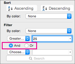
Depending on your choice, you may be offered additional criteria to select:
To
Click
Filter the table column or selection so that both criteria must be true
And.
Filter the table column or selection so that either or both criteria can be true
Or.
-
Click a cell in the range or table that you want to filter.
-
On the Data toolbar, select Filter.
-
Select the arrow
-
Under Filter, select Choose One, and then in the pop-up menu, do one of the following:
To filter for
Click
The beginning of a line of text
Begins With.
The end of a line of text
Ends With.
Cells that contain text but do not begin with letters
Does Not Begin With.
Cells that contain text but do not end with letters
Does Not End With.
-
In the box next to the pop-up menu, enter the text that you want to use.
-
Depending on your choice, you may be offered additional criteria to select:
To
Click
Filter the table column or selection so that both criteria must be true
And.
Filter the table column or selection so that either or both criteria can be true
Or.
Wildcard characters can be used to help you build criteria.
-
Click a cell in the range or table that you want to filter.
-
On the Data toolbar, select Filter.
-
Select the arrow
-
Under Filter, select Choose One, and select any option.
-
In the text box, type your criteria and include a wildcard character.
For example, if you wanted your filter to catch both the word "seat" and "seam", type sea?.
-
Do one of the following:
Use
To find
? (question mark)
Any single character
For example, sm?th finds "smith" and "smyth"
* (asterisk)
Any number of characters
For example, *east finds "Northeast" and "Southeast"
~ (tilde)
A question mark or an asterisk
For example, there~? finds "there?"
Do any of the following:
|
To |
Do this |
|---|---|
|
Remove specific filter criteria for a filter |
Select the arrow |
|
Remove all filters that are applied to a range or table |
Select the columns of the range or table that have filters applied, and then on the Data tab, select Filter. |
|
Remove filter arrows from or reapply filter arrows to a range or table |
Select the columns of the range or table that have filters applied, and then on the Data tab, select Filter. |
When you filter data, only the data that meets your criteria appears. The data that doesn't meet that criteria is hidden. After you filter data, you can copy, find, edit, format, chart, and print the subset of filtered data.
Table with Top 4 Items filter applied
Filters are additive. This means that each additional filter is based on the current filter and further reduces the subset of data. You can make complex filters by filtering on more than one value, more than one format, or more than one criteria. For example, you can filter on all numbers greater than 5 that are also below average. But some filters (top and bottom ten, above and below average) are based on the original range of cells. For example, when you filter the top ten values, you'll see the top ten values of the whole list, not the top ten values of the subset of the last filter.
In Excel, you can create three kinds of filters: by values, by a format, or by criteria. But each of these filter types is mutually exclusive. For example, you can filter by cell color or by a list of numbers, but not by both. You can filter by icon or by a custom filter, but not by both.
Filters hide extraneous data. In this manner, you can concentrate on just what you want to see. In contrast, when you sort data, the data is rearranged into some order. For more information about sorting, see Sort a list of data.
When you filter, consider the following guidelines:
-
Only the first 10,000 unique entries in a list appear in the filter window.
-
You can filter by more than one column. When you apply a filter to a column, the only filters available for other columns are the values visible in the currently filtered range.
-
You can apply filters to only one range of cells on a sheet at a time.
Note: When you use Find to search filtered data, only the data that is displayed is searched; data that is not displayed is not searched. To search all the data, clear all filters.
Need more help?
You can always ask an expert in the Excel Tech Community or get support in Communities.


Need more help?
Want more options?
Explore subscription benefits, browse training courses, learn how to secure your device, and more.


Communities help you ask and answer questions, give feedback, and hear from experts with rich knowledge.


