
If you're exploring charts in Excel and having a hard time figuring out which one is right for you, then you can try the Recommended Charts command on the Insert tab. Excel will analyze your data and make suggestions for you.
-
Select the data you want to use for your chart.
-
Click Insert > Recommended Charts.
-
On the Recommended Charts tab, scroll through the list of charts that Excel recommends for your data, and click any chart to see how your data will look.
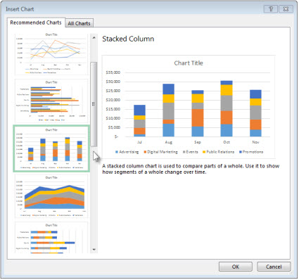
Tip: If you don’t see a chart you like, click All Charts to see all available chart types.
-
When you find the chart you like, click it > OK.
-
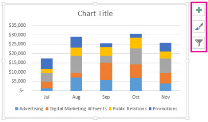
Use the Chart Elements, Chart Styles, and Chart Filters buttons next to the upper-right corner of the chart to add chart elements like axis titles or data labels, customize the look of your chart, or change the data that’s shown in the chart.
-
To access additional design and formatting features, click anywhere in the chart to add the Chart Tools to the ribbon, and then click the options you want on the Design and Format tabs.

-
Select the data you want to use for your chart.
-
Click Insert > Recommended Charts.
-
On the Recommended Charts tab, scroll through the list of charts that Excel recommends for your data, and click any chart to see how your data will look.
Tip: If you don’t see a chart you like, click All Charts to see all available chart types.
-
When you find the chart you like, click it > OK.
-
Use the Chart Elements, Chart Styles, and Chart Filters buttons next to the upper-right corner of the chart to add chart elements like axis titles or data labels, customize the look of your chart, or change the data that’s shown in the chart.
-
To access additional design and formatting features, click anywhere in the chart to add the Chart Tools to the ribbon, and then click the options you want on the Design and Format tabs.
Recommended charts in Excel for the web creates interesting visuals about your data in a task pane.
Note: Recommended charts are available to Microsoft 365 subscribers in English, French, Spanish, German, Simplified Chinese, and Japanese. If you are a Microsoft 365 subscriber, make sure you have the latest version of Office. To learn more about the different update channels for Office, see: Overview of update channels for Microsoft 365 Apps.
Get started
-
Select the data you want to use for your chart.
-
Click Insert > Recommended Charts.
-
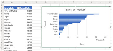
Choose a chart to insert from the Recommended Charts task pane, and select the + Insert Pivot Chart or + Insert Chart option.
-
If you choose the Pivot chart option, then Excel will insert a new worksheet for you with a PivotTable that is the data source for the Pivot Chart you selected. Each time you use the Insert Pivot Chart option, Excel will insert a new worksheet. If you choose the Insert Chart option, Excel will insert a chart directly on the worksheet with your source data.
Not sure how to get started?
If you're not sure how to get started, we'll give you some sample data you can experiment with.
-
Add a new worksheet -- You can right-click on any sheet tab, then select Insert.
-
Go to Insert > Recommended Charts, and Excel will load the Recommended Charts pane.
-
Select the Try sample data button.
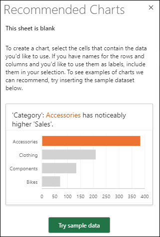
Excel will add some sample data to your worksheet, analyze it, then add recommended charts to the pane.
-
Follow the steps in the Get Started section to insert any of the recommended Pivot Charts or charts.
Need more help?
You can always ask an expert in the Excel Tech Community or get support in Communities.


