When you create a chart in Excel, it uses the information in the cell above each column or row of data as the legend name. You can change legend names by updating the information in those cells, or you can update the default legend name by using Select Data.
Note: If you create a chart without using row or column headers, Excel uses default names, starting with “Series 1.” You can learn more about how to create a chart to ensure your rows and columns are formatted properly.
In this article
Show the legend in your chart
-
Select the chart, click

-
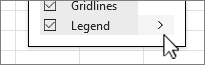
Optional. Select the > arrow to the right of Legend for options on where to place the legend in your chart.
Change the legend name in the excel data
-
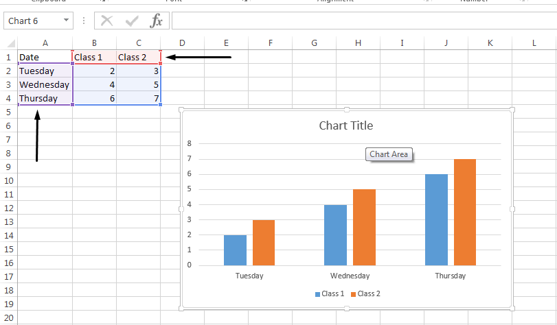
Select the cell in the workbook that contains the legend name you want to change.
Tip: You can first click your chart to see what cells within your data are included in your legend.
-
Type the new legend name in the selected cell, and press Enter. The legend name in the chart updates to the new legend name in your data.
-
Certain charts, such as Clustered Columns, also use the cells to the left of each row as legend names. You can edit legend names the same way.
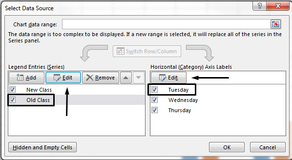
Change the legend name using select data
-
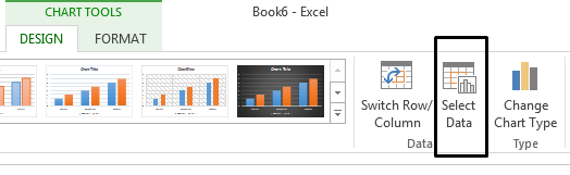
Select your chart and on the Chart Design tab, choose Select Data.
-
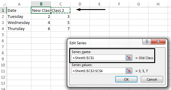
Choose on the legend name you want to change in the Select Data Source dialog box, and select Edit.
Note: You can update Legend Entries and Axis Label names from this view, and multiple Edit options might be available.
-
Type a legend name into the Series name text box, and click OK. The legend name in the chart changes to the new legend name.
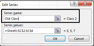
Note: This modifies your only chart legend names, not your cell data. Alternatively, you can select a different cell in your data to use as the legend name. Click inside the Series name text box, and select the cell within your data.