
In PivotTables, you can use summary functions in value fields to combine values from the underlying source data. If summary functions and custom calculations do not provide the results that you want, you can create your own formulas in calculated fields and calculated items. For example, you could add a calculated item with the formula for the sales commission, which could be different for each region. The PivotTable would then automatically include the commission in the subtotals and grand totals.
Another way to calculate is to use Measures in Power Pivot, which you create using a Data Analysis Expressions (DAX) formula. For more information, see Create a Measure in Power Pivot.
PivotTables provide ways to calculate data. Learn about the calculation methods that are available, how calculations are affected by the type of source data, and how to use formulas in PivotTables and PivotCharts.
To calculate values in a PivotTable, you can use any or all of the following types of calculation methods:
-
Summary functions in value fields The data in the values area summarize the underlying source data in the PivotTable. For example, the following source data:
-
Produces the following PivotTables and PivotCharts. If you create a PivotChart from the data in a PivotTable, the values in that PivotChart reflect the calculations in the associated PivotTable report.
-
In the PivotTable, the Month column field provides the items March and April. The Region row field provides the items North, South, East, and West. The value at the intersection of the April column and the North row is the total sales revenue from the records in the source data that have Month values of April and Region values of North.
-
In a PivotChart, the Region field might be a category field that shows North, South, East, and West as categories. The Month field could be a series field that shows the items March, April, and May as series represented in the legend. A Values field named Sum of Sales could contain data markers that represent the total revenue in each region for each month. For example, one data marker would represent, by its position on the vertical (value) axis, the total sales for April in the North region.
-
To calculate the value fields, the following summary functions are available for all types of source data except Online Analytical Processing (OLAP) source data.
Function
Summarizes
Sum
The sum of the values. This is the default function for numeric data.
Count
The number of data values. The Count summary function works the same as the COUNTA function. Count is the default function for data other than numbers.
Average
The average of the values.
Max
The largest value.
Min
The smallest value.
Product
The product of the values.
Count Nums
The number of data values that are numbers. The Count Nums summary function works the same as the COUNT function.
StDev
An estimate of the standard deviation of a population, where the sample is a subset of the entire population.
StDevp
The standard deviation of a population, where the population is all of the data to be summarized.
Var
An estimate of the variance of a population, where the sample is a subset of the entire population.
Varp
The variance of a population, where the population is all of the data to be summarized.
-
Custom calculations A custom calculation shows values based on other items or cells in the data area. For example, you could display values in the Sum of Sales data field as a percentage of March sales, or as a running total of the items in the Month field.
The following functions are available for custom calculations in value fields.
Function
Result
No Calculation
Displays the value that is entered in the field.
% of Grand Total
Displays values as a percentage of the grand total of all of the values or data points in the report.
% of Column Total
Displays all of the values in each column or series as a percentage of the total for the column or series.
% of Row Total
Displays the value in each row or category as a percentage of the total for the row or category.
% Of
Displays values as a percentage of the value of the Base item in the Base field.
% of Parent Row Total
Calculates values as follows:
(value for the item) / (value for the parent item on rows)
% of Parent Column Total
Calculates values as follows:
(value for the item) / (value for the parent item on columns)
% of Parent Total
Calculates values as follows:
(value for the item) / (value for the parent item of the selected Base field)
Difference From
Displays values as the difference from the value of the Base item in the Base field.
% Difference From
Displays values as the percentage difference from the value of the Base item in the Base field.
Running Total in
Displays the value for successive items in the Base field as a running total.
% Running Total in
Calculates the value for successive items in the Base field that are displayed as a running total as a percentage.
Rank Smallest to Largest
Displays the rank of selected values in a specific field, listing the smallest item in the field as 1, and each larger value will have a higher rank value.
Rank Largest to Smallest
Displays the rank of selected values in a specific field, listing the largest item in the field as 1, and each smaller value will have a higher rank value.
Index
Calculates values as follows:
((value in cell) x (Grand Total of Grand Totals)) / ((Grand Row Total) x (Grand Column Total))
-
Formulas If summary functions and custom calculations do not provide the results that you want, you can create your own formulas in calculated fields and calculated items. For example, you could add a calculated item with the formula for the sales commission, which could be different for each region. The report would then automatically include the commission in the subtotals and grand totals.
Calculations and options that are available in a report depend on whether the source data came from an OLAP database or a non-OLAP data source.
-
Calculations based on OLAP source data For PivotTables that are created from OLAP cubes, the summarized values are precalculated on the OLAP server before Excel displays the results. You cannot change how these precalculated values are calculated in the PivotTable. For example, you cannot change the summary function that is used to calculate data fields or subtotals, or add calculated fields or calculated items.
Also, if the OLAP server provides calculated fields, known as calculated members, you will see these fields in the PivotTable Field List. You will also see any calculated fields and calculated items that are created by macros that were written in Visual Basic for Applications (VBA) and stored in your workbook, but you won't be able to change these fields or items. If you need additional types of calculations, contact your OLAP database administrator.
For OLAP source data, you can include or exclude the values for hidden items when calculating subtotals and grand totals.
-
Calculations based on non-OLAP source data In PivotTables that are based on other types of external data or on worksheet data, Excel uses the Sum summary function to calculate value fields that contain numeric data, and the Count summary function to calculate data fields that contain text. You can choose a different summary function, such as, Average, Max, or Min, to further analyze and customize your data. You can also create your own formulas that use elements of the report or other worksheet data by creating a calculated field or a calculated item within a field.
You can create formulas only in reports that are based on a non-OLAP source data. You cannot use formulas in reports that are based on an OLAP database. When you use formulas in PivotTables, you should know about the following formula syntax rules and formula behavior:
-
PivotTable formula elements In formulas that you create for calculated fields and calculated items, you can use operators and expressions as you do in other worksheet formulas. You can use constants and refer to data from the report, but you cannot use cell references or defined names. You cannot use worksheet functions that require cell references or defined names as arguments, and you cannot use array functions.
-
Field and item names Excel uses field and item names to identify those elements of a report in your formulas. In the following example, the data in range C3:C9 is using the field name Dairy. A calculated item in the Type field that estimates sales for a new product based on Dairy sales could use a formula such as =Dairy * 115%.
Note: In a PivotChart, the field names are displayed in the PivotTable field list, and item names can be seen in each field drop-down list. Don't confuse these names with those you see in chart tips, which reflect series and data point names instead.
-
Formulas operate on sum totals, not individual records Formulas for calculated fields operate on the sum of the underlying data for any fields in the formula. For example, the calculated field formula =Sales * 1.2 multiplies the sum of the sales for each type and region by 1.2; it does not multiply each individual sale by 1.2 and then sum the multiplied amounts.
Formulas for calculated items operate on the individual records. For example, the calculated item formula =Dairy *115% multiplies each individual sale of Dairy times 115%, after which the multiplied amounts are summarized together in the Values area.
-
Spaces, numbers, and symbols in names In a name that includes more than one field, the fields can be in any order. In the example above, cells C6:D6 can be 'April North' or 'North April'. Use single quotation marks around names that are more than one word or that include numbers or symbols.
-
Totals Formulas cannot refer to totals (such as, March Total, April Total, and Grand Total in the example).
-
Field names in item references You can include the field name in a reference to an item. The item name must be in square brackets — for example, Region[North]. Use this format to avoid #NAME? errors when two items in two different fields in a report have the same name. For example, if a report has an item named Meat in the Type field and another item named Meat in the Category field, you can prevent #NAME? errors by referring to the items as Type[Meat] and Category[Meat].
-
Referring to items by position You can refer to an item by its position in the report as currently sorted and displayed. Type[1] is Dairy, and Type[2] is Seafood. The item referred to in this way can change whenever the positions of items change or different items are displayed or hidden. Hidden items are not counted in this index.
You can use relative positions to refer to items. The positions are determined relative to the calculated item that contains the formula. If South is the current region, Region[-1] is North; if North is the current region, Region[+1] is South. For example, a calculated item could use the formula =Region[-1] * 3%. If the position that you give is before the first item or after the last item in the field, the formula results in a #REF! error.
To use formulas in a PivotChart, you create the formulas in the associated PivotTable, where you can see the individual values that make up your data, and then you can view the results graphically in the PivotChart.
For example, the following PivotChart shows sales for each salesperson per region:
To see what sales would look like if they were increased by 10 percent, you could create a calculated field in the associated PivotTable that uses a formula such as =Sales * 110%.
The result immediately appears in the PivotChart, as shown in the following chart:
To see a separate data marker for sales in the North region minus a transportation cost of 8 percent, you could create a calculated item in the Region field with a formula such as =North – (North * 8%).
The resulting chart would look like this:
However, a calculated item that is created in the Salesperson field would appear as a series represented in the legend and appear in the chart as a data point in each category.
Important: You cannot create formulas in a PivotTable that is connected to an Online Analytical Processing (OLAP) data source.
Before you start, decide whether you want a calculated field or a calculated item within a field. Use a calculated field when you want to use the data from another field in your formula. Use a calculated item when you want your formula to use data from one or more specific items within a field.
For calculated items, you can enter different formulas cell by cell. For example, if a calculated item named OrangeCounty has a formula of =Oranges * .25 across all months, you can change the formula to =Oranges *.5 for June, July, and August.
If you have multiple calculated items or formulas, you can adjust the order of calculation.
Add a calculated field
-
Click the PivotTable.
This displays the PivotTable Tools, adding the Analyze and Design tabs.
-
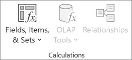
On the Analyze tab, in the Calculations group, click Fields, Items, & Sets, and then click Calculated Field.
-
In the Name box, type a name for the field.
-
In the Formula box, enter the formula for the field.
To use the data from another field in the formula, click the field in the Fields box, and then click Insert Field. For example, to calculate a 15% commission on each value in the Sales field, you could enter = Sales * 15%.
-
Click Add.
Add a calculated item to a field
-
Click the PivotTable.
This displays the PivotTable Tools, adding the Analyze and Design tabs.
-
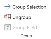
If items in the field are grouped, on the Analyze tab, in the Group group, click Ungroup.
-
Click the field where you want to add the calculated item.
-
On the Analyze tab, in the Calculations group, click Fields, Items, & Sets, and then click Calculated Item.
-
In the Name box, type a name for the calculated item.
-
In the Formula box, enter the formula for the item.
To use the data from an item in the formula, click the item in the Items list, and then click Insert Item (the item must be from the same field as the calculated item).
-
Click Add.
Enter different formulas cell by cell for calculated items
-
Click a cell for which you want to change the formula.
To change the formula for several cells, hold down CTRL and click the additional cells.
-
In the formula bar, type the changes to the formula.
Adjust the order of calculation for multiple calculated items or formulas
-
Click the PivotTable.
This displays the PivotTable Tools, adding the Analyze and Design tabs.
-
On the Analyze tab, in the Calculations group, click Fields, Items, & Sets, and then click Solve Order.
-
Click a formula, and then click Move Up or Move Down.
-
Continue until the formulas are in the order that you want them to be calculated.
You can display a list of all the formulas that are used in the current PivotTable.
-
Click the PivotTable.
This displays the PivotTable Tools, adding the Analyze and Design tabs.
-
On theAnalyze tab, in the Calculations group, click Fields, Items, & Sets, and then click List Formulas.
Before you edit a formula, determine whether that formula is in a calculated field or a calculated item. If the formula is in a calculated item, also determine whether the formula is the only one for the calculated item.
For calculated items, you can edit individual formulas for specific cells of a calculated item. For example, if a calculated item named OrangeCalc has a formula of =Oranges * .25 across all months, you can change the formula to =Oranges *.5 for June, July, and August.
Determine whether a formula is in a calculated field or a calculated item
-
Click the PivotTable.
This displays the PivotTable Tools, adding the Analyze and Design tabs.
-
On the Analyze tab, in the Calculations group, click Fields, Items, & Sets, and then click List Formulas.
-
In the list of formulas, find the formula that you want to change listed under Calculated Field or Calculated Item.
When there are multiple formulas for a calculated item, the default formula that was entered when the item was created has the calculated item name in column B. For additional formulas for a calculated item, column B contains both the calculated item name and the names of intersecting items.For example, you might have a default formula for a calculated item named MyItem, and another formula for this item identified as MyItem January Sales. In the PivotTable, you would find this formula in the Sales cell for the MyItem row and January column.
-
Continue by using one of the following editing methods.
Edit a calculated field formula
-
Click the PivotTable.
This displays the PivotTable Tools, adding the Analyze and Design tabs.
-
On the Analyze tab, in the Calculations group, click Fields, Items, & Sets, and then click Calculated Field.
-
In the Name box, select the calculated field for which you want to change the formula.
-
In the Formula box, edit the formula.
-
Click Modify.
Edit a single formula for a calculated item
-
Click the field that contains the calculated item.
-
On the Analyze tab, in the Calculations group, click Fields, Items, & Sets, and then click Calculated Item.
-
In the Name box, select the calculated item.
-
In the Formula box, edit the formula.
-
Click Modify.
Edit an individual formula for a specific cell of a calculated item
-
Click a cell for which you want to change the formula.
To change the formula for several cells, hold down CTRL and click the additional cells.
-
In the formula bar, type the changes to the formula.
Tip: If you have multiple calculated items or formulas, you can adjust the order of calculation. For more information, see Adjust the order of calculation for multiple calculated items or formulas.
Note: Deleting a PivotTable formula removes it permanently. If you do not want to remove a formula permanently, you can hide the field or item instead by dragging it out of the PivotTable.
-
Determine whether the formula is in a calculated field or a calculated item.
Calculated fields appear in the PivotTable Field List. Calculated items appear as items within other fields.
-
Do one of the following:
-
To delete a calculated field, click anywhere in the PivotTable.
-
To delete a calculated item, in the PivotTable, click the field that contains the item that you want to delete.
This displays the PivotTable Tools, adding the Analyze and Design tabs.
-
-
On the Analyze tab, in the Calculations group, click Fields, Items, & Sets, and then click Calculated Field or Calculated Item.
-
In the Name box, select the field or item that you want to delete.
-
Click Delete.
To summarize values in a PivotTable in Excel for the web, you can use summary functions like Sum, Count, and Average. The Sum function is used by default for numeric values in value fields. You can view and edit a PivotTable based on an OLAP data source, but you can’t create one in Excel for the web.
Here’s how to choose a different summary function:
-
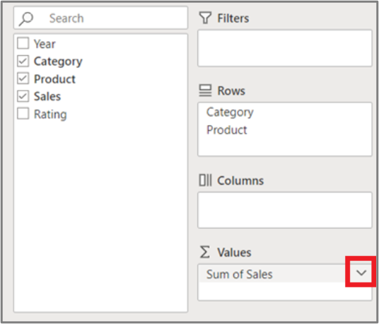
Click anywhere on the PivotTable, and then select PivotTable > Field List. You can also right-click the PivotTable and then select Show Field List.
-
In the PivotTable Fields list, under Values, click the arrow next to the value field.
-
Click Value Field Settings.
-
Pick the summary function you want and then click OK.
Note: Summary functions aren’t available in PivotTables that are based on Online Analytical Processing (OLAP) source data.
Use this summary function
To calculate
Sum
The sum of the values. It’s used by default for value fields that have numeric values.
Count
The number of nonempty values. The Count summary function works the same as the COUNTA function. Count is used by default for value fields that have nonnumeric values or blanks.
Average
The average of the values.
Max
The largest value.
Min
The smallest value.
Product
The product of the values.
Count Numbers
The number of values that contain numbers (not the same as Count, which includes nonempty values).
StDev
An estimate of the standard deviation of a population, where the sample is a subset of the entire population.
StDevp
The standard deviation of a population, where the population is all of the data to be summarized.
Var
An estimate of the variance of a population, where the sample is a subset of the entire population.
Varp
The variance of a population, where the population is all of the data to be summarized.
PivotTable on iPad is available to customers running Excel on iPad version 2.82.205.0 and above. To access this feature, please ensure your app is updated to the latest version through the App Store.
To summarize values in a PivotTable in Excel for iPad, you can use summary functions like Sum, Count, and Average. The Sum function is used by default for numeric values in value fields. You can view and edit a PivotTable based on an OLAP data source, but you can’t create one in Excel for iPad.
Here’s how to choose a different summary function:
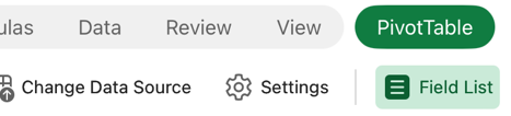
1. Tap anywhere in the PivotTable to show to the PivotTable tab, swipe left and select Field List to display the field list.
2. In the PivotTable Fields list, under Values, tap the ellipsis next to the value field.
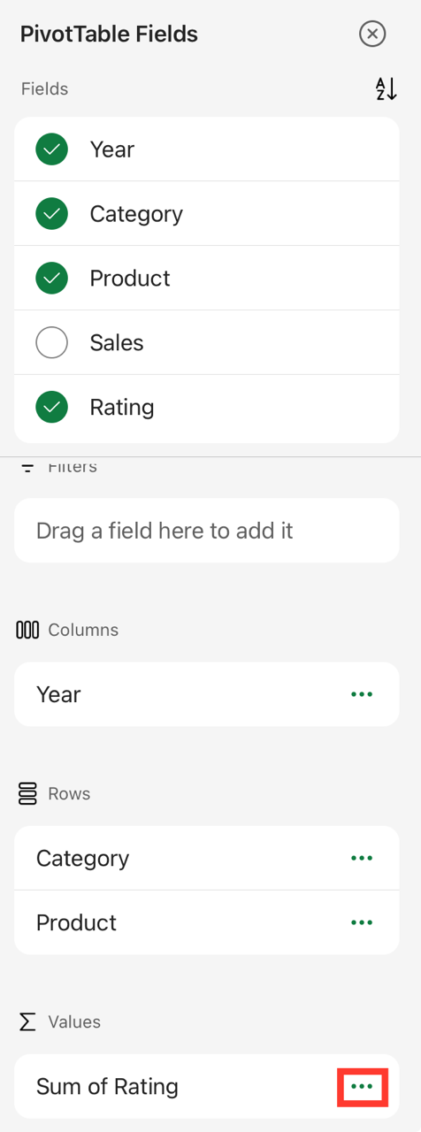
3. Tap Field Settings.
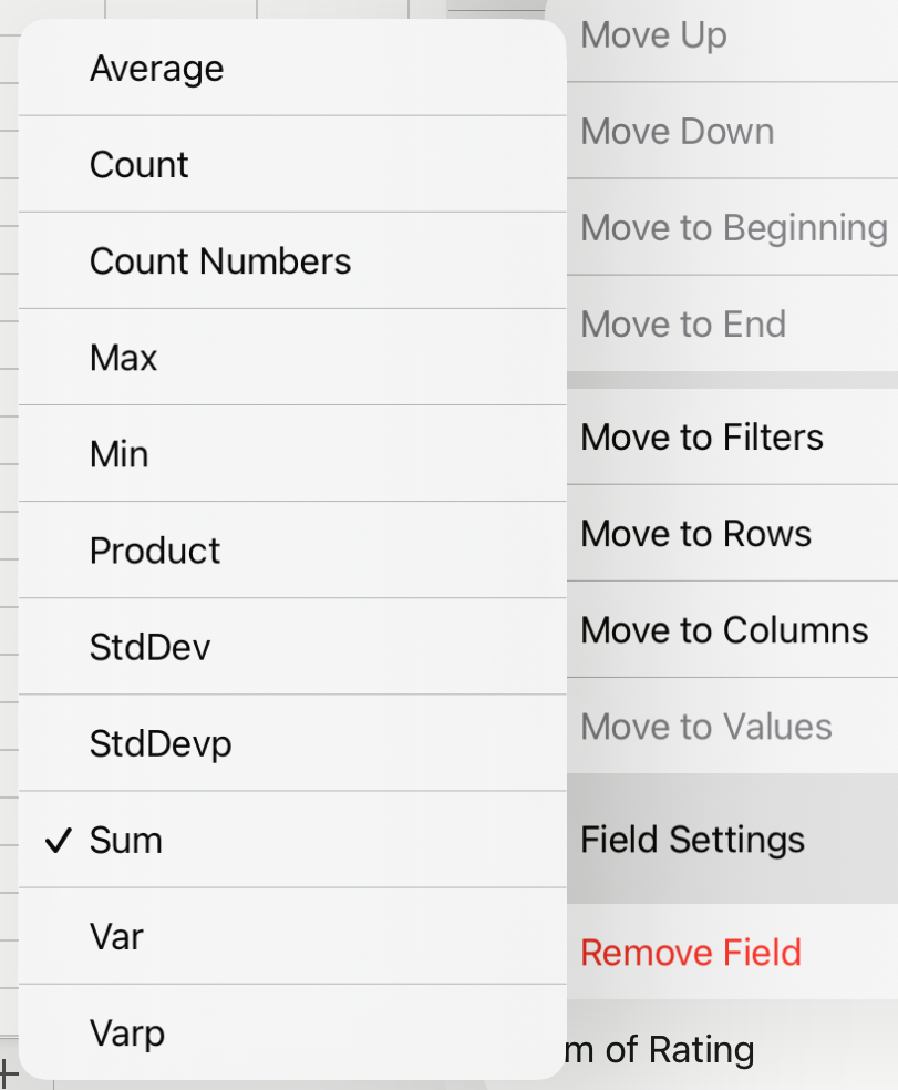
4. Check the summary function you want.
Note: Summary functions aren’t available in PivotTables that are based on Online Analytical Processing (OLAP) source data.
|
Use this summary function |
To calculate |
|---|---|
|
Sum |
The sum of the values. It’s used by default for value fields that have numeric values. |
|
Count |
The number of nonempty values. The Count summary function works the same as the COUNTA function. Count is used by default for value fields that have nonnumeric values or blanks. |
|
Average |
The average of the values. |
|
Max |
The largest value. |
|
Min |
The smallest value. |
|
Product |
The product of the values. |
|
Count Numbers |
The number of values that contain numbers (not the same as Count, which includes nonempty values). |
|
StDev |
An estimate of the standard deviation of a population, where the sample is a subset of the entire population. |
|
StDevp |
The standard deviation of a population, where the population is all of the data to be summarized. |
|
Var |
An estimate of the variance of a population, where the sample is a subset of the entire population. |
|
Varp |
The variance of a population, where the population is all of the data to be summarized. |
Need more help?
You can always ask an expert in the Excel Tech Community or get support in Communities.


