
Just by using the Power Query Editor, you have been creating Power Query formulas all along. Let's see how Power Query works by looking under the hood. You can learn how to update or add formulas just by watching the Power Query Editor in action. You can even roll your own formulas with the Advanced Editor.
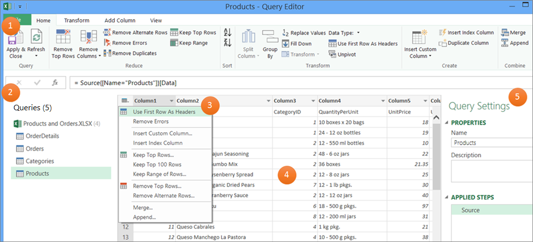
The Power Query Editor provides a data query and shaping experience for Excel that you can use to reshape data from many data sources. To display the Power Query Editor window, import data from external data sources in an Excel worksheet, select a cell in the data, and then select Query > Edit. The following is a summary of the main components.
-
The Power Query Editor ribbon that you use to shape your data
-
The Queries pane that you use to locate data sources and tables
-
Context menus that are convenient shortcuts to commands in the ribbon
-
The Data Preview that displays the results of the steps applied to the data
-
The Query Settings pane that lists properties and each step in the query
Behind the scenes, each step in a query is based on a formula that is visible in the formula bar.
There may be times when you want to modify or create a formula. Formulas use the Power Query Formula Language, which you can use to build both simple and complex expressions. For more information about syntax, arguments, remarks, functions, and examples, see Power Query M formula language.
Using a list of soccer championships as an example, use Power Query to take raw data that you found on a website and turn it into a well-formatted table. Watch how query steps and corresponding formulas are created for each task in the Query Settings pane under Applied Steps and in the Formula bar.

Procedure
-
To import the data, select Data > From Web, enter "http://en.wikipedia.org/wiki/UEFA_European_Football_Championship" in the URL box, and then select OK.
-
In the Navigator dialog box, select the Results [Edit] table on the left, and then select Transform Data at the bottom. The Power Query editor appears.
-
To change the default query name, in the Query Settings pane, under Properties, delete "Results [Edit]" and then enter "UEFA champs".
-
To remove unwanted columns, select the first, fourth, and fifth columns, and then select Home > Remove Column > Remove Other Columns.
-
To remove unwanted values, select Column1, select Home > Replace Values, enter "details" in the Values to Find box, and then select OK.
-
To remove rows that have the word "Year' in them, select the filter arrow in Column1, clear the check box next to "Year", and then select OK.
-
To rename the column headers, double-click each of them and then change "Column1" to "Year", "Column4" to "Winner", and "Column5" to "Final Score".
-
To save the query, select Home > Close & Load.
Result

The following table is a summary of each applied step and the corresponding formula.
|
Query step and task |
Formula |
|---|---|
|
Source Connect to a web data source |
= Web.Page(Web.Contents("http://en.wikipedia.org/wiki/UEFA_European_Football_Championship")) |
|
Navigation Select the table to connect |
=Source{2}[Data] |
|
Changed Type Change datatypes (which Power Query does automatically) |
= Table.TransformColumnTypes(Data2,{{"Column1", type text}, {"Column2", type text}, {"Column3", type text}, {"Column4", type text}, {"Column5", type text}, {"Column6", type text}, {"Column7", type text}, {"Column8", type text}, {"Column9", type text}, {"Column10", type text}, {"Column11", type text}, {"Column12", type text}}) |
|
Removed Other Columns Remove other columns to only display columns of interest |
= Table.SelectColumns(#"Changed Type",{"Column1", "Column4", "Column5"}) |
|
Replaced Value Replace values to clean up values in a selected column |
= Table.ReplaceValue(#"Removed Other Columns","Details","",Replacer.ReplaceText,{"Column1"}) |
|
Filtered Rows Filter values in a column |
= Table.SelectRows(#"Replaced Value", each ([Column1] <> "Year")) |
|
Renamed Columns Changed column headers to be meaningful |
= Table.RenameColumns(#"Filtered Rows",{{"Column1", "Year"}, {"Column4", "Winner"}, {"Column5", "Final Score"}}) |
Important Be careful editing the Source, Navigation, and Changed Type steps because they are created by Power Query to define and set up the data source.
Show or hide the formula bar
The formula bar is shown by default, but if it's not visible you can redisplay it.
-
Select View > Layout > Formula Bar.
Edit a formula in the formula bar
-
To open a query, locate one previously loaded from the Power Query Editor, select a cell in the data, and then select Query > Edit. For more information see Create, load, or edit a query in Excel.
-
In the Query Settings pane, under Applied Steps, select the step you want to edit.
-
In the formula bar, locate and change the parameter values, and then select the Enter

Before: = Table.SelectColumns(#"Changed Type",{"Column4", "Column1", "Column5"})
After:= Table.SelectColumns(#"Changed Type",{"Column2", "Column4", "Column1", "Column5"}) -
Select the Enter
-
To see the result in an Excel worksheet, select Home > Close & Load.
Create a formula in the formula bar
For a simple formula example, let’s convert a text value to proper case using the Text.Proper function.
-
To open a blank query, in Excel select Data > Get Data > From Other Sources > Blank Query. For more information see Create, load, or edit a query in Excel.
-
In the formula bar, enter =Text.Proper("text value"), and then select the Enter
The results display in Data Preview . -
To see the result in an Excel worksheet, select Home > Close & Load.
Result:

When you create a formula, Power Query validates the formula syntax. However, when you insert, reorder, or delete an intermediate step in a query you might potentially break a query. Always verify the results in Data Preview.
Important Be careful editing the Source, Navigation, and Changed Type steps because they are created by Power Query to define and set up the data source.
Edit a formula by using a dialog box
This method makes use of dialog boxes that vary depending on the step. You don't need to know the syntax of the formula.
-
To open a query, locate one previously loaded from the Power Query Editor, select a cell in the data, and then select Query > Edit. For more information see Create, load, or edit a query in Excel.
-
In the Query Settings pane, under Applied Steps, select the Edit Settings
-
In the dialog box, make your changes, and then select OK.

Insert a step
After you complete a query step that reshapes your data, a query step is added below the current query step. but when you insert a query step in the middle of the steps, an error might occur in subsequent steps. Power Query displays an Insert Step warning when you try to insert a new step and the new step alters fields, such as column names, that are used in any of the steps that follow the inserted step.
-
In the Query Settings pane, under Applied Steps, select the step you want to immediately precede the new step and its corresponding formula.
-
Select the Add Step

= <nameOfTheStepToReference>, such as =Production.WorkOrder. -
Type in the new formula using the format:
=Class.Function(ReferenceStep[,otherparameters])
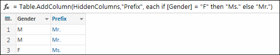
For example, assume you have a table with the column Gender and you want to add a column with the value “Ms.” or “Mr.”, depending on the person’s gender. The formula would be:
=Table.AddColumn(<ReferencedStep>, "Prefix", each if [Gender] = "F" then "Ms." else "Mr.")
Reorder a step
-
In the Queries Settings pane under Applied Steps, right click the step, and then select Move Up or Move Down.
Delete a step
-
Select the Delete

In this example, let’s convert the text in a column to proper case using a combination of formulas in the Advanced Editor.
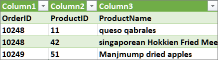
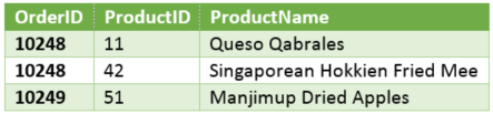
For example, you have an Excel table, called Orders, with a ProductName column that you want to convert to proper case.
Before:
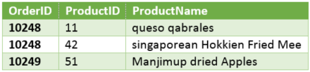
After:
When you create an advanced query, you create a series of query formula steps based on the let expression. Use the let expression to assign names and calculate values that are then referenced by the in clause, which defines the Step. This example returns the same result as the one in the "Create a formula in the formula bar" section.
let
Source = Text.Proper("hello world")
in
Source
You'll see that each step builds upon a previous step by referring to a step by name. As a reminder, the Power Query Formula Language is case-sensitive.
Phase 1: Open the Advanced Editor
-
In Excel, select Data > Get Data > Other Sources > Blank Query. For more information see Create, load, or edit a query in Excel.
-
In the Power Query Editor, select Home > Advanced Editor, which opens with a template of the let expression.

Phase 2: Define the data source
-
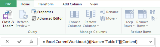
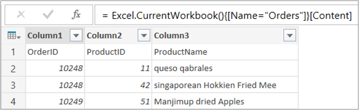
Create the let expression using the Excel.CurrentWorkbook function as follows:
let
Source = Excel.CurrentWorkbook(){[Name="Orders"]}[Content]
in
Source
-
To load the query to a worksheet, select Done, and then select Home > Close & Load > Close & Load.
Result:
Phase 3: Promote the first row to headers
-
To open the query, from the worksheet select a cell in the data, and then select Query > Edit. For more information see Create, load, or edit a query in Excel (Power Query).
-
In the Power Query Editor, select Home > Advanced Editor, which opens with the statement you created in Phase 2: Define the data source.
-
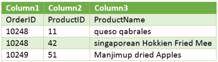
In the let expression, add #"First Row as Header" and Table.PromoteHeaders function as follows:
let
Source = Excel.CurrentWorkbook(){[Name="Orders"]}[Content],
#"First Row as Header" = Table.PromoteHeaders(Source)
in
#"First Row as Header" -
To load the query to a worksheet, select Done, and then select Home > Close & Load > Close & Load.
Result:
Phase 4: Change each value in a column to proper case
-
To open the query, from the worksheet select a cell in the data, and then select Query > Edit. For more information see Create, load, or edit a query in Excel.
-
In the Power Query Editor, select Home > Advanced Editor, which opens with the statement you created in Phase 3: Promote the first row to headers.
-
In the let expression, convert each ProductName column value to proper text by using the Table.TransformColumns function, referring to the previous "First Row as Header” query formula step, adding #"Capitalized Each Word" to the data source, and then assigning #"Capitalized Each Word" to the in result.
let
Source = Excel.CurrentWorkbook(){[Name="Orders"]}[Content],
#"First Row as Header" = Table.PromoteHeaders(Source),
#"Capitalized Each Word" = Table.TransformColumns(#"First Row as Header",{{"ProductName", Text.Proper}})
in
#"Capitalized Each Word" -
To load the query to a worksheet, select Done, and then select Home > Close & Load > Close & Load.
Result:
You can control the behavior of the formula bar in the Power Query Editor for all your workbooks.
Display or hide the formula bar
-
Select File > Options and Settings > Query Options.
-
In the left pane, under GLOBAL, select Power Query Editor.
-
In the right pane, under Layout, select or clear Display the Formula Bar.
Turn on or off M Intellisense
-
Select File > Options and Settings > Query Options .
-
In the left pane, under GLOBAL, select Power Query Editor.
-
In the right pane, under Formula, select or clear Enable M Intellisense in the formula bar, advanced editor, and custom column dialog.
Note Changing this setting will take effect the next time you open the Power Query Editor window.
See Also
Create and invoke a custom function
Using the Applied Steps list (docs.com)
Using custom functions (docs.com)


