
Note: This article has done its job, and will be retiring soon. To prevent "Page not found" woes, we're removing links we know about. If you've created links to this page, please remove them, and together we'll keep the web connected.
You can perform calculations and logical comparisons in a table by using formulas. Word automatically updates the results of formulas in a document when you open the document. Word also updates the results when you use the command Update field.
Note: Formulas in tables are a type of field code. For more information about field codes, see Field codes in Word.
In this article
Open the Formula dialog box
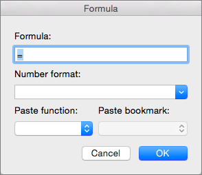
To add or modify formulas in Word, you must open the Formula dialog box. In the Formula dialog box, you can edit formulas, select number formats, select functions to paste into a formula, and paste bookmarks.
The procedures in this topic describe using the Table menu to open the Formula dialog box, but you can also open the Formula dialog box by clicking Formula on the Layout tab.
-
Place the cursor in the table cell where you want to create or modify a formula.
When you place the cursor in a table cell, or select text in a table, Word displays the Table Design and Layout tabs, which are normally hidden.
-
Do one of the following:
-
If your Word window is wide, click Formula, which appears directly the ribbon.
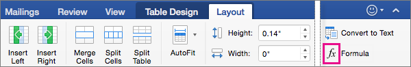
-
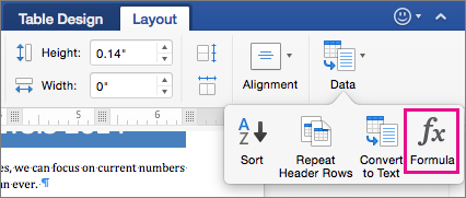
If your Word window is narrow, first click Data to open its menu, and then click Formula.
-
On the Table menu, click Formula.
-
Insert a formula in a table cell
-
Select the table cell where you want your result.
If the cell is not empty, delete its contents.
-
On the Layout tab, click Formula.
Alternatively, on the Table menu, click Formula.
-
Use the Formula dialog box to create your formula.
You can type in the Formula box, select a number format from the Number Format list, and paste in functions and bookmarks using the Paste Function and Paste Bookmark lists.
Update formula results
Word calculates the result of a formula when you insert it in a document and when Word opens the document that contains the formula.
You can also cause Word to recalculate the result of one or more specific formulas.
-
Select the formulas that you want to update.
You can select multiple formulas by holding down the

-
Control + click the formula, and then click Update field.
Examples: Sum numbers in a table by using positional arguments
You can use positional arguments (LEFT, RIGHT, ABOVE, BELOW) with these functions:
-
AVERAGE
-
COUNT
-
MAX
-
MIN
-
PRODUCT
-
SUM
As an example, consider the following procedure for adding numbers by using the SUM function and positional arguments.
Important: To avoid an error while summing in a table by using positional arguments, type a zero (0) in any empty cell that will be included in the calculation.
-
Select the table cell where you want your result.
-
If the cell is not empty, delete its contents.
-
On the Layout tab, click Formula.
Alternatively, on the Table menu, click Formula.
-
Identify which numbers you want to add, and then enter the corresponding formula shown in the following table.
To add the numbers…
Type this in the Formula box
Above the cell
=SUM(ABOVE)
Below the cell
=SUM(BELOW)
Above and below the cell
=SUM(ABOVE,BELOW)
Left of the cell
=SUM(LEFT)
Right of the cell
=SUM(RIGHT)
Left and right of the cell
=SUM(LEFT,RIGHT)
Left of and above the cell
=SUM(LEFT,ABOVE)
Right of and above the cell
=SUM(RIGHT,ABOVE)
Left of and below the cell
=SUM(LEFT,BELOW)
Right of and below the cell
=SUM(RIGHT,BELOW)
-
Click OK.
Available functions
Note: Formulas that use positional arguments (for example, LEFT) do not include values in header rows.
The functions described in the following table are available for use in table formulas.
|
Function |
What it does |
Example |
Returns |
|
ABS() |
Calculates the absolute value of the value inside the parentheses |
=ABS(-22) |
22 |
|
AND() |
Evaluates whether the arguments inside the parentheses are all TRUE. |
=AND(SUM(LEFT)<10,SUM(ABOVE)>=5) |
1, if the sum of the values to the left of the formula (in the same row) is less than 10 and the sum of the values above the formula (in the same column, excluding any header cell) is greater than or equal to 5; 0 otherwise. |
|
AVERAGE() |
Calculates the average of items identified inside the parentheses. |
=AVERAGE(RIGHT) |
The average of all values to the right of the formula cell, in the same row. |
|
COUNT() |
Calculates the count of items identified inside the parentheses. |
=COUNT(LEFT) |
The number of values to the left of the formula cell, in the same row. |
|
DEFINED() |
Evaluates whether the argument inside the parentheses is defined. Returns 1 if the argument has been defined and evaluates without error, 0 if the argument has not been defined or returns an error. |
=DEFINED(gross_income) |
1, if gross_income has been defined and evaluates without error; 0 otherwise. |
|
FALSE |
Takes no arguments. Always returns 0. |
=FALSE |
0 |
|
IF() |
Evaluates the first argument. Returns the second argument if the first argument is true; returns the third argument if the first argument is false. Note: Requires exactly three arguments. |
=IF(SUM(LEFT)>=10,10,0) |
10, if the sum of values to the left of the formula is at least 10; 0 otherwise. |
|
INT() |
Rounds the value inside the parentheses down to the nearest integer. |
=INT(5.67) |
5 |
|
MAX() |
Returns the maximum value of the items identified inside the parentheses. |
=MAX(ABOVE) |
The maximum value found in the cells above the formula (excluding any header rows). |
|
MIN() |
Returns the minimum value of the items identified inside the parentheses. |
=MIN(ABOVE) |
The minimum value found in the cells above the formula (excluding any header rows). |
|
MOD() |
Takes two arguments (must be numbers or evaluate to numbers). Returns the remainder after the second argument is divided by the first. If the remainder is 0 (zero), returns 0.0 |
=MOD(4,2) |
0.0 |
|
NOT() |
Takes one argument. Evaluates whether the argument is true. Returns 0 if the argument is true, 1 if the argument is false. Mostly used inside an IF formula. |
=NOT(1=1) |
0 |
|
OR() |
Takes two arguments. If either is true, returns 1. If both are false, returns 0. Mostly used inside an IF formula. |
=OR(1=1,1=5) |
1 |
|
PRODUCT() |
Calculates the product of items identified inside the parentheses. |
=PRODUCT(LEFT) |
The product of multiplying all the values found in the cells to the left of the formula. |
|
ROUND() |
Takes two arguments (first argument must be a number or evaluate to a number; second argument must be an integer or evaluate to an integer). Rounds the first argument to the number of digits specified by the second argument. If the second argument is greater than zero (0), first argument is rounded down to the specified number of digits. If second argument is zero (0), first argument is rounded down to the nearest integer. If second argument is negative, first argument is rounded down to the left of the decimal. |
=ROUND(123.456, 2) =ROUND(123.456, 0) =ROUND(123.456, -2) |
123.46 123 100 |
|
SIGN() |
Takes one argument that must either be a number or evaluate to a number. Evaluates whether the item identified inside the parentheses if greater than, equal to, or less than zero (0). Returns 1 if greater than zero, 0 if zero, -1 if less than zero. |
=SIGN(-11) |
-1 |
|
SUM() |
Calculates the sum of items identified inside the parentheses. |
=SUM(RIGHT) |
The sum of the values of the cells to the right of the formula. |
|
TRUE() |
Takes one argument. Evaluates whether the argument is true. Returns 1 if the argument is true, 0 if the argument is false. Mostly used inside an IF formula. |
=TRUE(1=0) |
0 |
Use bookmarknames or cell references in a formula
You can refer to a bookmarked cell by using its bookmark name in a formula. For example, if you have bookmarked a cell that contains or evaluates to a number with the bookmark name gross_income, the formula =ROUND(gross_income,0) rounds the value of that cell down to the nearest integer.
You can also use column and row references in a formula. There are two reference styles: RnCn and A1.
Note: The cell that contains the formula is not included in a calculation that uses a reference. If the cell is part of the reference, it is ignored.
RnCn references
You can refer to a table row, column, or cell in a formula by using the RnCn reference convention. In this convention, Rn refers to the nth row, and Cn refers to the nth column. For example, R1C2 refers to the cell that is in first row and the second column.
The following table contains examples of the RnCn reference style.
|
To refer to… |
…use this reference style |
|
An entire column |
Cn |
|
An entire row |
Rn |
|
A specific cell |
RnCn |
|
The row that contains the formula |
R |
|
The column that contains the formula |
C |
|
All the cells between two specified cells |
RnCn:RnCn |
|
A cell in a bookmarked table |
Bookmark_name RnCn |
|
A range of cells in a bookmarked table |
Bookmark_name RnCn:RnCn |
A1 references
You can refer to a cell, a set of cells, or a range of cells by using the A1 reference convention. In this convention, the letter refers to the cell’s column and the number refers to the cell’s row. The first column in a table is column A; the first row is row 1.
The following table contains examples of the A1 reference style.
|
To refer to… |
…use this reference |
|
The cell in the first column and the second row |
A2 |
|
The first two cells in the first row |
A1,B1 |
|
All the cells in the first column and the first two cells in the second column |
A1:B2 |


