
Conditional formatting quickly highlights important information in a spreadsheet. But sometimes the built-in formatting rules don’t go quite far enough. Adding your own formula to a conditional formatting rule gives it a power boost to help you do things the built-in rules can’t do.
For example, let’s say you track your dental patients’ birthdays to see whose is coming up and then mark them as having received a Happy Birthday greeting from you.
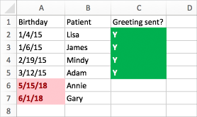
In this worksheet, we see the information we want by using conditional formatting, driven by two rules that each contain a formula. The first rule, in column A, formats future birthdays, and the rule in column C formats cells as soon as “Y” is entered, indicating that the birthday greeting has been sent.
To create the first rule:
-
Select cells A2 through A7. Do this by dragging from A2 to A7.
-
On the Home tab, click Conditional Formatting > New Rule.
-
In the Style box, click Classic.
-
Under the Classic box, click to select Format only top or bottom ranked values, and change it to Use a formula to determine which cells to format.
-
In the next box, type the formula: =A2>TODAY()
The formula uses the TODAY function to see if the dates in column A are greater than today (in the future). If so, the cells are formatted.
-
On the Format with box, click custom format.
-
In the Format Cells dialog box, click the Font tab.
-
In the Color box, select Red. In the Font style box, select Bold.
-
Click OK until the dialog boxes are closed.
The formatting is applied to column A.
To create the second rule:
-
Select cells C2 through C7.
-
On the Home tab, click Conditional Formatting > New Rule.
-
In the Style box, click Classic.
-
Under the Classic box, click to select Format only top or bottom ranked values, and change it to Use a formula to determine which cells to format.
-
In the next box, type the formula: =C2="Y"
The formula tests to see if the cells in column C contain “Y” (the quotation marks around the Y tell Excel that this is text). If so, the cells are formatted.
-
On the Format with box, click custom format.
-
At the top, click the Font tab.
-
In the Color box, select White. In the Font Style box, select Bold.
-
At the top, click the Fill tab, and then for Background color, select Green.
-
Click OK until the dialog boxes are closed.
The formatting is applied to column C.
Try it out
In the examples above, we used very simple formulas for conditional formatting. Experiment on your own and use other formulas you are familiar with.
Here's one more example if you want to take it to the next level. Type the following data table into your workbook. Start in cell A1. Then, select cells D2:D11, and create a new conditional formatting rule that uses this formula:
=COUNTIF($D$2:$D$11,D2)>1
When you create the rule, make sure it applies to cells D2:D11. Set a color format to be applied to cells that match the criteria (that is, there is more than one instance of a city in the D column – Seattle and Spokane).
|
First |
Last |
Phone |
City |
|
Annik |
Stahl |
555-1213 |
Seattle |
|
Josh |
Barnhill |
555-1214 |
Portland |
|
Colin |
Wilcox |
555-1215 |
Spokane |
|
Harry |
Miller |
555-1216 |
Edmonds |
|
Jonathan |
Foster |
555-1217 |
Atlanta |
|
Erin |
Hagens |
555-1218 |
Spokane |
|
Jeff |
Phillips |
555-1219 |
Charleston |
|
Gordon |
Hee |
555-1220 |
Youngstown |
|
Yossi |
Ran |
555-1221 |
Seattle |
|
Anna |
Bedecs |
555-1222 |
San Francisco |


