
If you create a custom number format for a 16-digit credit card number (such as ################ or ####-####-####-####), Excel changes the last digit to a zero because Excel changes any digits past the fifteenth place to zeros.
In addition, Excel displays the number in exponential notation, replacing part of the number with E+n, where E (which signifies exponent) multiplies the preceding number by 10 to the nth power. To successfully display a 16-digit credit card number in full, you must format the number as text.
For security purposes, you can obscure all except the last few digits of a credit card number by using a formula that includes the CONCATENATE, RIGHT, and REPT functions.
Display credit card numbers in full
-
Select the cell or range of cells that you want to format.
How to select a cell or a range
To select
Do this
A single cell
Click the cell, or press the arrow keys to move to the cell.
A range of cells
Click the first cell in the range, and then drag to the last cell, or hold down SHIFT while you press the arrow keys to extend the selection.
You can also select the first cell in the range, and then press F8 to extend the selection by using the arrow keys. To stop extending the selection, press F8 again.
A large range of cells
Click the first cell in the range, and then hold down SHIFT while you click the last cell in the range. You can scroll to make the last cell visible.
All cells on a worksheet
Click the Select All button.

To select the entire worksheet, you can also press CTRL+A.
Note: If the worksheet contains data, CTRL+A selects the current region. Pressing CTRL+A a second time selects the entire worksheet.
Nonadjacent cells or cell ranges
Select the first cell or range of cells, and then hold down CTRL while you select the other cells or ranges.
You can also select the first cell or range of cells, and then press SHIFT+F8 to add another nonadjacent cell or range to the selection. To stop adding cells or ranges to the selection, press SHIFT+F8 again.
Note: You cannot cancel the selection of a cell or range of cells in a nonadjacent selection without canceling the entire selection.
An entire row or column
Click the row or column heading.
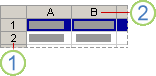
1. Row heading
2. Column heading
You can also select cells in a row or column by selecting the first cell and then pressing CTRL+SHIFT+ARROW key (RIGHT ARROW or LEFT ARROW for rows, UP ARROW or DOWN ARROW for columns).
Note: If the row or column contains data, CTRL+SHIFT+ARROW key selects the row or column to the last used cell. Pressing CTRL+SHIFT+ARROW key a second time selects the entire row or column.
Adjacent rows or columns
Drag across the row or column headings. Or select the first row or column; then hold down SHIFT while you select the last row or column.
Nonadjacent rows or columns
Click the column or row heading of the first row or column in your selection; then hold down CTRL while you click the column or row headings of other rows or columns that you want to add to the selection.
The first or last cell in a row or column
Select a cell in the row or column, and then press CTRL+ARROW key (RIGHT ARROW or LEFT ARROW for rows, UP ARROW or DOWN ARROW for columns).
The first or last cell on a worksheet or in a Microsoft Office Excel table
Press CTRL+HOME to select the first cell on the worksheet or in an Excel list.
Press CTRL+END to select the last cell on the worksheet or in an Excel list that contains data or formatting.
Cells to the last used cell on the worksheet (lower-right corner)
Select the first cell, and then press CTRL+SHIFT+END to extend the selection of cells to the last used cell on the worksheet (lower-right corner).
Cells to the beginning of the worksheet
Select the first cell, and then press CTRL+SHIFT+HOME to extend the selection of cells to the beginning of the worksheet.
More or fewer cells than the active selection
Hold down SHIFT while you click the last cell that you want to include in the new selection. The rectangular range between the active cell and the cell you click becomes the new selection.
Tip: To cancel a selection of cells, click any cell on the worksheet.
Tip: You can also select empty cells, and then enter numbers after you format the cells as text. Those numbers will be formatted as text.
-
Click the Home tab, and then click the Dialog Box Launcher
-
In the Category box, click Text.
Note: If you don't see the Text option, use the scroll bar to scroll to the end of the list.

Tip: To include other characters (such as dashes) in numbers that are stored as text, you can include them when you type the credit card numbers.
For common security measures, you may want to display only the last few digits of a credit card number and replace the rest of the digits with asterisks or other characters. You can do this by using a formula that includes the CONCATENATE, REPT, and RIGHT functions.
The following procedure uses example data to show how you can display only the last four numbers of a credit card number. After you copy the formula to your worksheet, you can adjust it to display your own credit card numbers in a similar manner.
-
Create a blank workbook or worksheet.
-
In this Help article, select the following example data without the row and column headers.
A
B
1
Type
Data
2
Credit Card Number
5555-5555-5555-5555
3
Formula
Description (Result)
4
=CONCATENATE(REPT("****-",3), RIGHT(B2,4))
Repeats the "****-" text string three times and combines the result with the last four digits of the credit card number (****-****-****-5555)
-
How to select example data
-
Click in front of the text in cell A1, and then drag the pointer across the cells to select all the text.
-

-
-
To copy the selected data, press CTRL+C.
-
In the worksheet, select cell A1.
-
To paste the copied data, press CTRL+V.
-
To switch between viewing the result and viewing the formula that returns the result, on the Formulas tab, in the Formula Auditing group, click Show Formulas.
Tip: Keyboard shortcut: You can also press CTRL+` (grave accent).
-
Notes:
-
To prevent other people from viewing the entire credit card number, you can first hide the column that contains that number (column B in the example data), and then protect the worksheet so that unauthorized users cannot unhide the data. For more information, see Hide or display rows and columns and Protect worksheet or workbook elements.
-
For more information about these functions, see CONCATENATE, REPT, and RIGHT, RIGHTB.


