
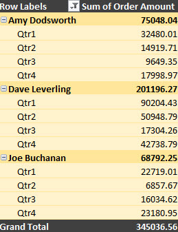
If you don’t like the look of your PivotTable after you create it, you can pick a different style. For example, when you have a lot of data in your PivotTable, it may help to show banded rows or columns for easy scanning or to highlight important data to make it stand out.
-
Click anywhere in the PivotTable to show the PivotTable Tools on the ribbon.
-
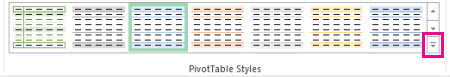
Click Design, and then click the More button in the PivotTable Styles gallery to see all available styles.
-
Pick the style you want to use.
-
If you don’t see a style you like, you can create your own. Click New PivotTable Style at the bottom of the gallery, provide a name for your custom style, and then pick the options you want.
Tip: If you want to change the PivotTable form and the way that fields, columns, rows, subtotals, empty cells, and lines are displayed, you can design the layout and format of a PivotTable.
Show banded rows for ease of scanning
-
Click anywhere in the PivotTable to show the PivotTable Tools on the ribbon.
-
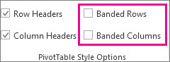
Click Design > Banded Rows (or Banded Columns).
You can view and interact with the data in PivotTables, but the PivotTable tools you’d need to make changes to the style of the PivotTable aren’t available in Excel for the web. You will need the desktop version of Excel to be able to do that. See Change the style of your PivotTable.
PivotTable on iPad is available to customers running Excel on iPad version 2.82.205.0 and above. To access this feature, please ensure your app is updated to the latest version through the App Store.
-
Tap anywhere in the PivotTable to show to the PivotTable tab on the ribbon.
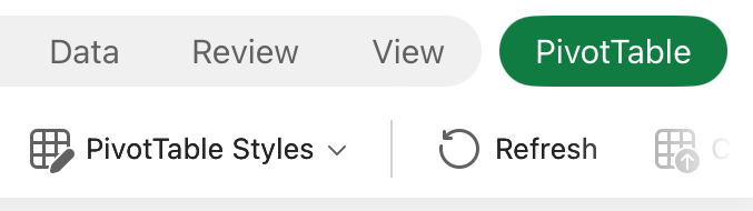
-
Tap PivotTable Styles, and then scroll up in the gallery to see all available styles.
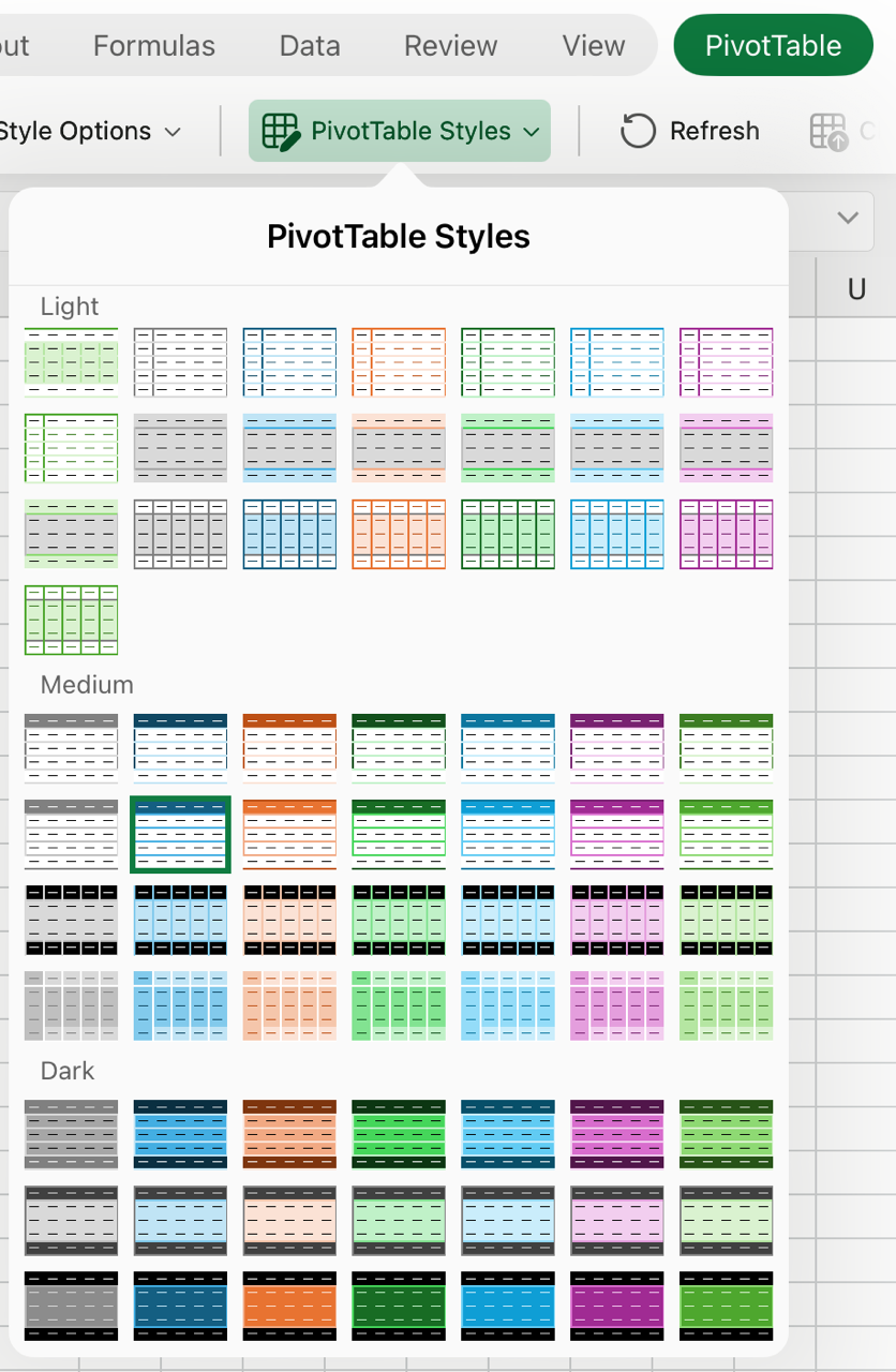
-
Pick the style you want to use.
-
If you want to change the PivotTable form and the way that fields, columns, rows, subtotals, empty cells, and lines are displayed, you can design the layout and format of a PivotTable.
Show banded rows for ease of scanning
-
Tap anywhere in the PivotTable to show to the PivotTable tab on the ribbon.
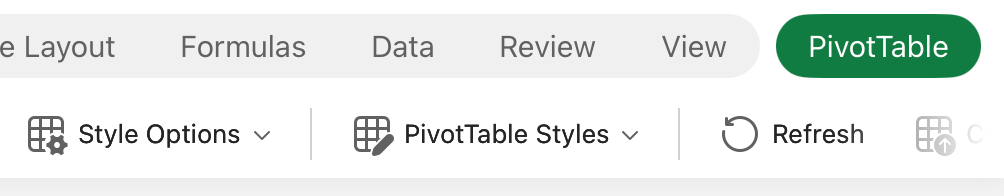
-
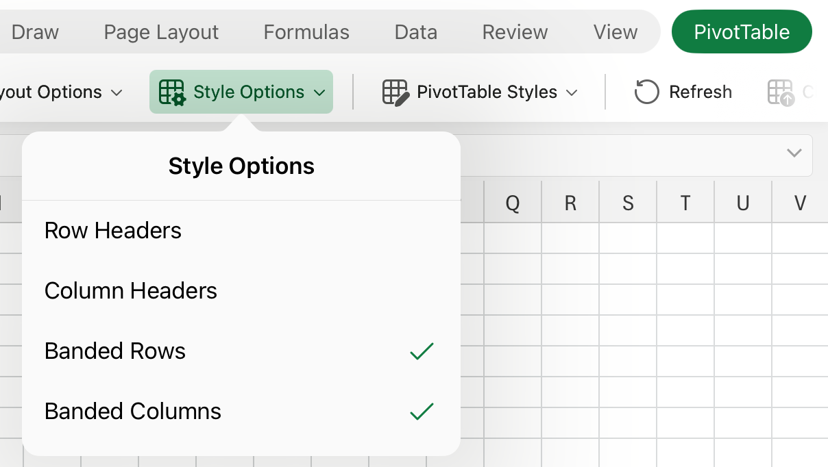
Tap Style Options > Banded Rows (or Banded Columns).
Need more help?
You can always ask an expert in the Excel Tech Community or get support in Communities.
See Also
Create a PivotTable to analyze worksheet data
Create a PivotTable to analyze external data
Create a PivotTable to analyze data in multiple tables


