
After creating a PivotTable and adding the fields that you want to analyze, you may want to enhance the report layout and format to make the data easier to read and scan for details. To change the layout of a PivotTable, you can change the PivotTable form and the way that fields, columns, rows, subtotals, empty cells and lines are displayed. To change the format of the PivotTable, you can apply a predefined style, banded rows, and conditional formatting.
To make substantial layout changes to a PivotTable or its various fields, you can use one of three forms:
-
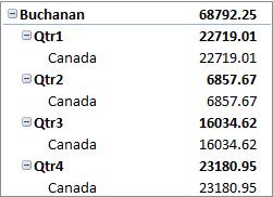
Compact form displays items from different row area fields in one column and uses indentation to distinguish between the items from different fields. Row labels take up less space in compact form, which leaves more room for numeric data. Expand and Collapse buttons are displayed so that you can display or hide details in compact form. Compact form is saves space and makes the PivotTable more readable and is therefore specified as the default layout form for PivotTables.
-
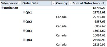
Tabular form displays one column per field and provides space for field headers.
-
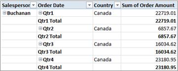
Outline form is similar to tabular form but it can display subtotals at the top of every group because items in the next column are displayed one row below the current item.
-
Click anywhere in the PivotTable.
This displays the PivotTable Tools, tab on the ribbon.
-
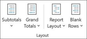
On the Design tab, in the Layout group, click Report Layout, and then do one of the following:
-
To keep related data from spreading horizontally off of the screen and to help minimize scrolling, click Show in Compact Form.
In compact form, fields are contained in one column and indented to show the nested column relationship.
-
To outline the data in the classic PivotTable style, click Show in Outline Form.
-
To see all data in a traditional table format and to easily copy cells to another worksheet, click Show in Tabular Form.
-
-
In the PivotTable, select a row field.
This displays the PivotTable Tools tab on the ribbon.
You can also double-click the row field in outline or tabular form, and continue with step 3.
-
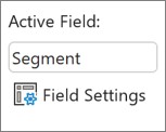
On the Analyze or Options tab, in the Active Field group, click Field Settings.
-
In the Field Settings dialog box, click the Layout & Print tab, and then under Layout, do one of the following:
-
To show field items in outline form, click Show item labels in outline form.
-
To display or hide labels from the next field in the same column in compact form, click Show item labels in outline form, and then select Display labels from the next field in the same column (compact form).
-
To show field items in table-like form, click Show item labels in tabular form.
-
To get the final layout results that you want, you can add, rearrange, and remove fields by using the PivotTable Field List.
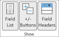
If you don't see the PivotTable Field List, make sure that the PivotTable is selected. If you still don't see the PivotTable Field List, on the Options tab, in the Show/Hide group, click Field List.
If you don't see the fields that you want to use in the PivotTable Field List, you may need to refresh the PivotTable to display any new fields, calculated fields, measures, calculated measures, or dimensions that you have added since the last operation. On the Options tab, in the Data group, click Refresh.
For more information about working with the PivotTable Field List, see Use the Field List to arrange fields in a PivotTable.
Do one or more of the following:
-
Select the check box next to each field name in the field section. The field is placed in a default area of the layout section, but you can rearrange the fields if you want.
By default, text fields are added to the Row Labels area, numeric fields are added to the Values area, and Online Analytical Processing (OLAP) date and time hierarchies are added to the Column Labels area.
-
Right-click the field name and then select the appropriate command — Add to Report Filter, Add to Column Label, Add to Row Label, or Add to Values — to place the field in a specific area of the layout section.
-
Click and hold a field name, and then drag the field between the field section and an area in the layout section.
In a PivotTable that is based on data in an Excel worksheet or external data from a non-OLAP source data, you may want to add the same field more than once to the Values area so that you can display different calculations by using the Show Values As feature. For example, you may want to compare calculations side-by-side, such as gross and net profit margins, minimum and maximum sales, or customer counts and percentage of total customers. For more information, see Show different calculations in PivotTable value fields.
-
Click and hold a field name in the field section, and then drag the field to the Values area in the layout section.
-
Repeat step 1 as many times as you want to copy the field.
-
In each copied field, change the summary function or custom calculation the way you want.
Notes:
-
When you add two or more fields to the Values area, whether they are copies of the same field or different fields, the Field List automatically adds a Values Column label to the Values area. You can use this field to move the field positions up and down within the Values area. You can even move the Values Column label to the Column Labels area or Row Labels areas. However, you can’t move the Values Column label to the Report Filters area.
-
You can add a field only once to either the Report Filter, Row Labels, or Column Labels areas, whether the data type is numeric or non-numeric. If you try to add the same field more than once — for example to the Row Labels and the Column Labels areas in the layout section — the field is automatically removed from the original area and put in the new area.
-
Another way to add the same field to the Values area is by using a formula (also called a calculated column) that uses that same field in the formula.
-
You cannot add the same field more than once in a PivotTable that is based on an OLAP data source.
-
You can rearrange existing fields or reposition those fields by using one of the four areas at the bottom of the layout section:
|
PivotTable report |
Description |
PivotChart |
Description |
|---|---|---|---|
|
Values |
Use to display summary numeric data. |
Values |
Use to display summary numeric data. |
|
Row Labels |
Use to display fields as rows on the side of the report. A row lower in position is nested within another row immediately above it. |
Axis Field (Categories) |
Use to display fields as an axis in the chart. |
|
Column Labels |
Use to display fields as columns at the top of the report. A column lower in position is nested within another column immediately above it. |
Legend Fields (Series) Labels |
Use to display fields in the legend of the chart. |
|
Report Filter |
Use to filter the entire report based on the selected item in the report filter. |
Report Filter |
Use to filter the entire report based on the selected item in the report filter. |
To rearrange fields, click the field name in one of the areas, and then select one of the following commands:
|
Select this |
To |
|---|---|
|
Move Up |
Move the field up one position in the area. |
|
Move Down |
Move the field down position in the area. |
|
Move to Beginning |
Move the field to the beginning of the area. |
|
Move to End |
Move the field to the end of the area. |
|
Move to Report Filter |
Move the field to the Report Filter area. |
|
Move to Row Labels |
Move the field to the Row Labels area. |
|
Move to Column Labels |
Move the field to the Column Labels area. |
|
Move to Values |
Move the field to the Values area. |
|
Value Field Settings, Field Settings |
Display the Field Settings or Value Field Settings dialog boxes. For more information about each setting, click the Help button |

You can also click and hold a field name, and then drag the field between the field and layout sections, and between the different areas.
-
Click the PivotTable.
This displays the PivotTable Tools tab on the ribbon.
-
To display the PivotTable Field List, if necessary, on the Analyze or Options tab, in the Show group, click Field List. You can also right click on the PivotTable and select Show Field List.
-
To remove a field, in the PivotTable Field List, do one of the following:
-
In the PivotTable Field List, clear the check box next to the field name.
Note: Clearing a check box in the Field List removes all instances of the field from the report.
-
In a Layout area, click the field name, and then click Remove Field.
-
Click and hold a field name in the layout section, and then drag it outside the PivotTable Field List.
-
To further refine the layout of a PivotTable, you can make changes that affect the layout of columns, rows, and subtotals, such as displaying subtotals above rows or turning column headers off. You can also rearrange individual items within a row or column.
Turn column and row field headers on or off
-
Click the PivotTable.
This displays the PivotTable Tools tab on the ribbon.
-
To switch between showing and hiding field headers, on the Analyze or Options tab, in the Show group, click Field Headers.
Display subtotals above or below their rows
-
In the PivotTable, select the row field for which you want to display subtotals.
This displays the PivotTable Tools tab on the ribbon.
Tip: In outline or tabular form, you can also double-click the row field, and then continue with step 3.
-
On the Analyze or Options tab, in the Active Field group, click Field Settings.
-
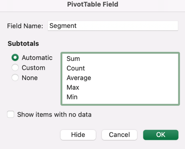
In the Field Settings dialog box, on the Subtotals & Filters tab, under the Subtotals, click Automatic or Custom.
Note: If None is selected, subtotals are turned off.
-
On the Layout & Print tab, under Layout, click Show item labels in outline form, and then do one of the following:
-
To display subtotals above the subtotaled rows, select the Display subtotals at the top of each group check box. This option is selected by default.
-
To display subtotals below the subtotaled rows, clear the Display subtotals at the top of each group check box.
-
Change the order of row or column items
Do any of the following:
-
In the PivotTable, right-click the row or column label or the item in a label, point to Move, and then use one of the commands on the Move menu to move the item to another location.
-
Select the row or column label item that you want to move, and then point to the bottom border of the cell. When the pointer becomes a four-headed pointer, drag the item to a new position. The following illustration shows how to move a row item by dragging.
Adjust column widths on refresh
-
Click anywhere in the PivotTable.
This displays the PivotTable Tools tab on the ribbon.
-
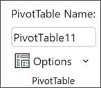
On the Analyze or Options tab, in the PivotTable group, click Options.
-
In the PivotTable Options dialog box, on the Layout & Format tab, under Format, do one of the following:
-
To automatically fit the PivotTable columns to the size of the widest text or number value, select the Autofit column widths on update check box.
-
To keep the current PivotTable column width, clear the Autofit column widths on update check box.
-
Move a column to the row labels area or a row to the column labels area
You might want to move a column field to the row labels area or a row field to the column labels area to optimize the layout and readability of the PivotTable. When you move a column to a row or a row to a column, you are transposing the vertical or horizontal orientation of the field. This operation is also called "pivoting" a row or column.
Use a right click command
Do any of the following:
-
Right-click a row field, point to Move <field name>, and then click Move <field name> To Columns.
-
Right-click a column field, and then click Move <field name> to Rows.
Use drag and drop
-
Switch to classic mode by placing the pointer on the PivotTable, selecting PivotTable Analyze > Options, selecting the Display tab, and then selecting Classic PivotTable layout.
-
Drag a row or column field to a different area. The following illustration shows how to move a column field to the row labels area.
a. Click a column field
b. Drag it to the row area
c. Sport becomes a row field like Region
Merge or unmerge cells for outer row and column items
You can merge cells for row and column items in order to center the items horizontally and vertically, or to unmerge cells in order to left-justify items in the outer row and column fields at the top of the item group.
-
Click anywhere in the PivotTable.
This displays the PivotTable Tools tab on the ribbon.
-
On the Options tab, in the PivotTable group, click Options.
-
In the PivotTable Options dialog box, click the Layout & Format tab, and then under Layout, select or clear the Merge and center cells with labels check box.
Note: You cannot use the Merge Cells check box under the Alignment tab in a PivotTable.
There may be times when your PivotTable data contains blank cells, blank lines, or errors, and you want to change the way they are displayed.
Change how errors and empty cells are displayed
-
Click anywhere in the PivotTable.
This displays the PivotTable Tools tab on the ribbon.
-
On the Analyze or Options tab, in the PivotTable group, click Options.
-
In the PivotTable Optionsdialog box, click the Layout & Format tab, and then under Format, do one or more of the following:
-
To change the error display, select the For error values show check box. In the box, type the value that you want to display instead of errors. To display errors as blank cells, delete any characters in the box.
-
To change the display of empty cells, select the For empty cells show check box, and then type the value that you want to display in empty cells in the text box.
Tip: To display blank cells, delete any characters in the box. To display zeros, clear the check box.
-
Display or hide blank lines after rows or items
For rows, do the following:
-
In the PivotTable, select a row field.
This displays the PivotTable Tools tab on the ribbon.
Tip: In outline or tabular form, you can also double-click the row field, and then continue with step 3.
-
On the Analyze or Options tab, in the Active Field group, click Field Settings.
-
In the Field Settings dialog box, on the Layout & Print tab, under Layout, select or clear the Insert blank line after each item label check box.
For items, do the following:
-
In the PivotTable, select the item you want.
This displays the PivotTable Tools tab on the ribbon.
-
On the Design tab, in the Layout group, click Blank Rows, and then select the Insert Blank Line after Each Item Label or Remove Blank Line after Each Item Label check box.
Note: You can apply character and cell formatting to the blank lines, but you cannot enter data in them.
Change how items and labels with no data are shown
-
Click anywhere in the PivotTable.
This displays the PivotTable Tools tab on the ribbon.
-
On the Analyze or Options tab, in the PivotTable group, click Options.
-
On the Display tab, under Display, do one or more of the following:
-
To show items with no data on rows, select or clear the Show items with no data on rows check box to display or hide row items that have no values.
Note: This setting is only available for an Online Analytical Processing (OLAP) data source.
-
To show items with no data on columns, select or clear the Show items with no data on columns check box to display or hide column items that have no values.
Note: This setting is only available for an OLAP data source.
-
To display item labels when no fields are in the values area, select or clear the Display item labels when no fields are in the values area check box to display or hide item labels when there are no fields in the value area.
-
You can choose from a wide variety of PivotTable styles in the gallery. In addition, you can control the banding behavior of a report. Changing the number format of a field is a quick way to apply a consistent format throughout a report. You can also add or remove banding (alternating a darker and lighter background) of rows and columns. Banding can make it easier to read and scan data.
Apply a style to format a PivotTable
You can quickly change the look and format of a PivotTable by using one of numerous predefined PivotTable styles (or quick styles).
-
Click anywhere in the PivotTable.
This displays the PivotTable Tools tab on the ribbon.
-
On the Design tab, in the PivotTable Styles group, do any of the following:
-
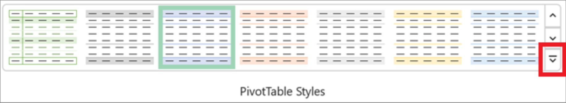
Click a visible PivotTable style or scroll through the gallery to see additional styles.
-
To see all of the available styles, click the More button at the bottom of the scroll bar.
If you want to create your own custom PivotTable style, click New PivotTable Style at the bottom of the gallery to display the New PivotTable Style dialog box.
-
Apply banding to change the format of a PivotTable
-
Click anywhere in the PivotTable.
This displays the PivotTable Tools tab on the ribbon.
-
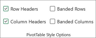
On the Design tab, in the PivotTable Style Options group, do one of the following:
-
To alternate each row with a lighter and darker color format, click Banded Rows.
-
To alternate each column with a lighter and darker color format, click Banded Columns.
-
To include row headers in the banding style, click Row Headers.
-
To include column headers in the banding style, click Column Headers.
-
Remove a style or banding format from a PivotTable
-
Click anywhere in the PivotTable.
This displays the PivotTable Tools tab on the ribbon.
-
On the Design tab, in the PivotTable Styles group, click the More button at the bottom of the scroll bar to see all of the available styles, and then click Clear at the bottom of the gallery.
Conditionally format data in a PivotTable
Use a conditional format to help you visually explore and analyze data, detect critical issues, and identify patterns and trends. Conditional formatting helps you answer specific questions about your data. There are important differences to understand when you use conditional formatting on a PivotTable:
-
If you change the layout of the PivotTable by filtering, hiding levels, collapsing and expanding levels, or moving a field, the conditional format is maintained as long as the fields in the underlying data are not removed.
-
The scope of the conditional format for fields in the Values area can be based on the data hierarchy and is determined by all the visible children (the next lower level in a hierarchy) of a parent (the next higher level in a hierarchy) on rows for one or more columns, or columns for one or more rows.
Note: In the data hierarchy, children do not inherit conditional formatting from the parent, and the parent does not inherit conditional formatting from the children.
-
There are three methods for scoping the conditional format of fields in the Values area: by selection, by corresponding field, and by value field.
For more information, see Apply conditional formatting.
Change the number format for a field
-
In the PivotTable, select the field of interest.
This displays the PivotTable Tools tab on the ribbon.
-
On the Analyze or Options tab in the Active Field group, click Field Settings.
The Field Settings dialog box displays labels and report filters; the Values Field Settings dialog box displays values.
-
Click Number Format at the bottom of the dialog box.
-
In the Format Cells dialog box, in the Category list, click the number format that you want to use.
-
Select the options that you prefer, and then click OK twice.
You can also right-click a value field, and then click Number Format.
Include OLAP server formatting
If you are connected to a Microsoft SQL Server Analysis Services Online Analytical Processing (OLAP) database, you can specify what OLAP server formats to retrieve and display with the data.
-
Click anywhere in the PivotTable.
This displays the PivotTable Tools tab on the ribbon.
-
On the Analyze or Options tab, in the Data group, click Change Data Source, and then click Connection Properties.
-
In the Connection Properties dialog box, on the Usage tab, and then under the OLAP Server Formatting section, do one of the following:
-
To enable or disable number formatting, such as currency, dates, and times, select or clear the Number Format check box.
-
To enable or disable font styles, such as bold, italics, underline, and strikethrough, select or clear the Font Style check box.
-
To enable or disable fill colors, select or clear the Fill Color check box.
-
To enable or disable text colors, select or clear the Text Color check box.
-
Preserve or discard formatting
-
Click anywhere in the PivotTable.
This displays the PivotTable Tools tab on the ribbon.
-
On the Analyze or Options tab, in the PivotTable group, click Options.
-
On the Layout & Format tab, under Format, do one of the following:
-
To save the PivotTable layout and format so that it is used each time that you perform an operation on the PivotTable, select the Preserve cell formatting on update check box.
-
To discard the PivotTable layout and format and resort to the default layout and format each time that you perform an operation on the PivotTable, clear the Preserve cell formatting on update check box.
Note: While this option also affects the PivotChart formatting, trendlines, data labels, error bars, and other changes to specific data series are not preserved.
-
Use the PivotTable Settings pane to make changes to your PivotTable's layout and formatting.
-
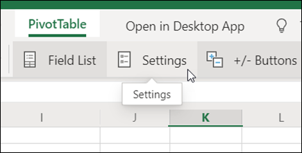
With the PivotTable selected, on the ribbon, click PivotTable > Settings.
-
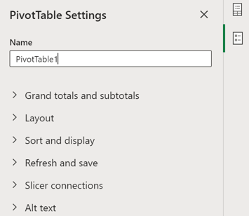
In the PivotTable Settings pane, adjust any of the following settings:
Note: The Slicer section only appears if the there is a slicer connected to your PivotTable.
To show grand totals
-
Select or clear Rows, Columns, or both.
To show subtotals
-
Select Don't show to hide any subtotals.
-
Select On top to display them above the values they summarize.
-
Select On bottom to display them below the values they summarize.
To place fields from Rows area
Select Separate columns to provide individual filters for each Rows field, or Single column to combine the Rows fields in one filter.
To show or hide item labels
Select Repeat or Don't repeat to choose whether item labels appear for each item or just once per item label value.
To add a blank line after each item
Select Show or Don't Show.
To autofit columns widths on refresh
Select to automatically resize the columns to fit the data whenever the PivotTable is refreshed.
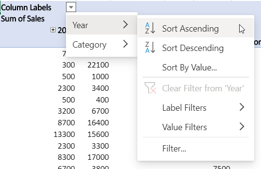
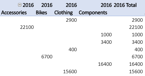
To show expand/collapse buttons
Select to show the expand/collapse buttons for groups of columns with the same value. For example, if your PivotTable has annual sales data for a set of products, you might have a group of columns for each value of Year.
To show error values
Select to display the value in the text box for cells containing errors.
To show empty cells
Select to display the value in the text box for cells with empty values. Otherwise, Excel displays a default value.
To save source data with file
Select to include the PivotTable's source data in the Excel file when you save. Note that this could result in a fairly large file.
To refresh data on file open
Select to have Excel refresh PivotTable data each time the file is opened.
To add a title
Provide a brief title to help people who use screen readers know what is depicted by your PivotTable.
To add a description
Provide several sentences with more details about the PivotTable contents or data source to help people who use screen readers understand the purpose of your PivotTable.
To make substantial layout changes to a PivotTable or its various fields, you can use one of three forms:
-
Compact form displays items from different row area fields in one column and uses indentation to distinguish between the items from different fields. Row labels take up less space in compact form, which leaves more room for numeric data. Expand and Collapse buttons are displayed so that you can display or hide details in compact form. Compact form is saves space and makes the PivotTable more readable and is therefore specified as the default layout form for PivotTables.
-
Tabular form displays one column per field and provides space for field headers.
-
Outline form is similar to tabular form but it can display subtotals at the top of every group because items in the next column are displayed one row below the current item.
-
Click anywhere in the PivotTable.
This displays the PivotTable Tools, tab on the ribbon.
-
On the Design tab, in the Layout group, click Report Layout, and then do one of the following:
-
To keep related data from spreading horizontally off of the screen and to help minimize scrolling, click Show in Compact Form.
In compact form, fields are contained in one column and indented to show the nested column relationship.
-
To outline the data in the classic PivotTable style, click Show in Outline Form.
-
To see all data in a traditional table format and to easily copy cells to another worksheet, click Show in Tabular Form.
-
To get the final layout results that you want, you can add, rearrange, and remove fields by using the PivotTable Field List.
If you don't see the PivotTable Field List, make sure that the PivotTable is selected. If you still don't see the PivotTable Field List, on the Options tab, in the Show/Hide group, click Field List.
If you don't see the fields that you want to use in the PivotTable Field List, you may need to refresh the PivotTable to display any new fields, calculated fields, measures, calculated measures, or dimensions that you have added since the last operation. On the Options tab, in the Data group, click Refresh.
For more information about working with the PivotTable Field List, see Use the Field List to arrange fields in a PivotTable.
Do one or more of the following:
-
Select the check box next to each field name in the field section. The field is placed in a default area of the layout section, but you can rearrange the fields if you want.
By default, text fields are added to the Row Labels area, numeric fields are added to the Values area, and Online Analytical Processing (OLAP) date and time hierarchies are added to the Column Labels area.
-
Right-click the field name and then select the appropriate command — Add to Report Filter, Add to Column Label, Add to Row Label, or Add to Values — to place the field in a specific area of the layout section.
-
Click and hold a field name, and then drag the field between the field section and an area in the layout section.
In a PivotTable that is based on data in an Excel worksheet or external data from a non-OLAP source data, you may want to add the same field more than once to the Values area so that you can display different calculations by using the Show Values As feature. For example, you may want to compare calculations side-by-side, such as gross and net profit margins, minimum and maximum sales, or customer counts and percentage of total customers. For more information, see Show different calculations in PivotTable value fields.
-
Click and hold a field name in the field section, and then drag the field to the Values area in the layout section.
-
Repeat step 1 as many times as you want to copy the field.
-
In each copied field, change the summary function or custom calculation the way you want.
Notes:
-
When you add two or more fields to the Values area, whether they are copies of the same field or different fields, the Field List automatically adds a Values Column label to the Values area. You can use this field to move the field positions up and down within the Values area. You can even move the Values Column label to the Column Labels area or Row Labels areas. However, you can’t move the Values Column label to the Report Filters area.
-
You can add a field only once to either the Report Filter, Row Labels, or Column Labels areas, whether the data type is numeric or non-numeric. If you try to add the same field more than once — for example to the Row Labels and the Column Labels areas in the layout section — the field is automatically removed from the original area and put in the new area.
-
Another way to add the same field to the Values area is by using a formula (also called a calculated column) that uses that same field in the formula.
-
You cannot add the same field more than once in a PivotTable that is based on an OLAP data source.
-
You can rearrange existing fields or reposition those fields by using one of the four areas at the bottom of the layout section:
|
PivotTable report |
Description |
PivotChart |
Description |
|---|---|---|---|
|
Values |
Use to display summary numeric data. |
Values |
Use to display summary numeric data. |
|
Row Labels |
Use to display fields as rows on the side of the report. A row lower in position is nested within another row immediately above it. |
Axis Field (Categories) |
Use to display fields as an axis in the chart. |
|
Column Labels |
Use to display fields as columns at the top of the report. A column lower in position is nested within another column immediately above it. |
Legend Fields (Series) Labels |
Use to display fields in the legend of the chart. |
|
Report Filter |
Use to filter the entire report based on the selected item in the report filter. |
Report Filter |
Use to filter the entire report based on the selected item in the report filter. |
To rearrange fields, click the field name in one of the areas, and then select one of the following commands:
|
Select this |
To |
|---|---|
|
Move Up |
Move the field up one position in the area. |
|
Move Down |
Move the field down position in the area. |
|
Move to Beginning |
Move the field to the beginning of the area. |
|
Move to End |
Move the field to the end of the area. |
|
Move to Report Filter |
Move the field to the Report Filter area. |
|
Move to Row Labels |
Move the field to the Row Labels area. |
|
Move to Column Labels |
Move the field to the Column Labels area. |
|
Move to Values |
Move the field to the Values area. |
|
Value Field Settings, Field Settings |
Display the Field Settings or Value Field Settings dialog boxes. For more information about each setting, click the Help button |
You can also click and hold a field name, and then drag the field between the field and layout sections, and between the different areas.
-
Click the PivotTable.
This displays the PivotTable Tools tab on the ribbon.
-
To display the PivotTable Field List, if necessary, on the Analyze or Options tab, in the Show group, click Field List. You can also right click on the PivotTable and select Show Field List.
-
To remove a field, in the PivotTable Field List, do one of the following:
-
In the PivotTable Field List, clear the check box next to the field name.
Note: Clearing a check box in the Field List removes all instances of the field from the report.
-
In a Layout area, click the field name, and then click Remove Field.
-
Click and hold a field name in the layout section, and then drag it outside the PivotTable Field List.
-
To further refine the layout of a PivotTable, you can make changes that affect the layout of columns, rows, and subtotals, such as displaying subtotals above rows or turning column headers off. You can also rearrange individual items within a row or column.
Turn column and row field headers on or off
-
Click the PivotTable.
This displays the PivotTable Tools tab on the ribbon.
-
To switch between showing and hiding field headers, on the Analyze or Options tab, in the Show group, click Field Headers.
Display subtotals above or below their rows
-
In the PivotTable, select the row field for which you want to display subtotals.
This displays the PivotTable Tools tab on the ribbon.
Tip: In outline or tabular form, you can also double-click the row field, and then continue with step 3.
-
On the Analyze or Options tab, in the Active Field group, click Field Settings.
-
In the Field Settings dialog box, on the Subtotals & Filters tab, under the Subtotals, click Automatic or Custom.
Note: If None is selected, subtotals are turned off.
-
On the Layout & Print tab, under Layout, click Show item labels in outline form, and then do one of the following:
-
To display subtotals above the subtotaled rows, select the Display subtotals at the top of each group check box. This option is selected by default.
-
To display subtotals below the subtotaled rows, clear the Display subtotals at the top of each group check box.
-
Change the order of row or column items
Do any of the following:
-
In the PivotTable, right-click the row or column label or the item in a label, point to Move, and then use one of the commands on the Move menu to move the item to another location.
-
Select the row or column label item that you want to move, and then point to the bottom border of the cell. When the pointer becomes a four-headed pointer, drag the item to a new position. The following illustration shows how to move a row item by dragging.
Adjust column widths on refresh
-
Click anywhere in the PivotTable.
This displays the PivotTable Tools tab on the ribbon.
-
On the Analyze or Options tab, in the PivotTable group, click Options.
-
In the PivotTable Options dialog box, on the Layout & Format tab, under Format, do one of the following:
-
To automatically fit the PivotTable columns to the size of the widest text or number value, select the Autofit column widths on update check box.
-
To keep the current PivotTable column width, clear the Autofit column widths on update check box.
-
Move a column to the row labels area or a row to the column labels area
You might want to move a column field to the row labels area or a row field to the column labels area to optimize the layout and readability of the PivotTable. When you move a column to a row or a row to a column, you are transposing the vertical or horizontal orientation of the field. This operation is also called "pivoting" a row or column.
Do any of the following:
-
Right-click a row field, point to Move <field name>, and then click Move <field name> To Columns.
-
Right-click a column field, and then click Move <field name> to Rows.
-
Drag a row or column field to a different area. The following illustration shows how to move a column field to the row labels area.
1. Click a column field
2. Drag it to the row area
3. Sport becomes a row field like Region
Merge or unmerge cells for outer row and column items
You can merge cells for row and column items in order to center the items horizontally and vertically, or to unmerge cells in order to left-justify items in the outer row and column fields at the top of the item group.
-
Click anywhere in the PivotTable.
This displays the PivotTable Tools tab on the ribbon.
-
On the Options tab, in the PivotTable group, click Options.
-
In the PivotTable Options dialog box, click the Layout & Format tab, and then under Layout, select or clear the Merge and center cells with labels check box.
Note: You cannot use the Merge Cells check box under the Alignment tab in a PivotTable.
There may be times when your PivotTable data contains blank cells, blank lines, or errors, and you want to change the way they are displayed.
Change how errors and empty cells are displayed
-
Click anywhere in the PivotTable.
This displays the PivotTable Tools tab on the ribbon.
-
On the Analyze or Options tab, in the PivotTable group, click Options.
-
In the PivotTable Options dialog box, click the Layout & Format tab, and then under Format, do one or more of the following:
-
To change the error display, select the For error values show check box. In the box, type the value that you want to display instead of errors. To display errors as blank cells, delete any characters in the box.
-
To change the display of empty cells, select the For empty cells show check box, and then type the value that you want to display in empty cells in the text box.
Tip: To display blank cells, delete any characters in the box. To display zeros, clear the check box.
-
Change how items and labels with no data are shown
-
Click anywhere in the PivotTable.
This displays the PivotTable Tools tab on the ribbon.
-
On the Analyze or Options tab, in the PivotTable group, click Options.
-
On the Display tab, under Display, do one or more of the following:
-
To show items with no data on rows, select or clear the Show items with no data on rows check box to display or hide row items that have no values.
Note: This setting is only available for an Online Analytical Processing (OLAP) data source.
-
To show items with no data on columns, select or clear the Show items with no data on columns check box to display or hide column items that have no values.
Note: This setting is only available for an OLAP data source.
-
You can choose from a wide variety of PivotTable styles in the gallery. In addition, you can control the banding behavior of a report. Changing the number format of a field is a quick way to apply a consistent format throughout a report. You can also add or remove banding (alternating a darker and lighter background) of rows and columns. Banding can make it easier to read and scan data.
Apply a style to format a PivotTable
You can quickly change the look and format of a PivotTable by using one of numerous predefined PivotTable styles (or quick styles).
-
Click anywhere in the PivotTable.
This displays the PivotTable Tools tab on the ribbon.
-
On the Design tab, in the PivotTable Styles group, do any of the following:
-
Click a visible PivotTable style or scroll through the gallery to see additional styles.
-
To see all of the available styles, click the More button at the bottom of the scroll bar.
If you want to create your own custom PivotTable style, click New PivotTable Style at the bottom of the gallery to display the New PivotTable Style dialog box.
-
Apply banding to change the format of a PivotTable
-
Click anywhere in the PivotTable.
This displays the PivotTable Tools tab on the ribbon.
-
On the Design tab, in the PivotTable Style Options group, do one of the following:
-
To alternate each row with a lighter and darker color format, click Banded Rows.
-
To alternate each column with a lighter and darker color format, click Banded Columns.
-
To include row headers in the banding style, click Row Headers.
-
To include column headers in the banding style, click Column Headers.
-
Remove a style or banding format from a PivotTable
-
Click anywhere in the PivotTable.
This displays the PivotTable Tools tab on the ribbon.
-
On the Design tab, in the PivotTable Styles group, click the More button at the bottom of the scroll bar to see all of the available styles, and then click Clear at the bottom of the gallery.
Conditionally format data in a PivotTable
Use a conditional format to help you visually explore and analyze data, detect critical issues, and identify patterns and trends. Conditional formatting helps you answer specific questions about your data. There are important differences to understand when you use conditional formatting on a PivotTable:
-
If you change the layout of the PivotTable by filtering, hiding levels, collapsing and expanding levels, or moving a field, the conditional format is maintained as long as the fields in the underlying data are not removed.
-
The scope of the conditional format for fields in the Values area can be based on the data hierarchy and is determined by all the visible children (the next lower level in a hierarchy) of a parent (the next higher level in a hierarchy) on rows for one or more columns, or columns for one or more rows.
Note: In the data hierarchy, children do not inherit conditional formatting from the parent, and the parent does not inherit conditional formatting from the children.
-
There are three methods for scoping the conditional format of fields in the Values area: by selection, by corresponding field, and by value field.
For more information, see Apply conditional formatting.
Include OLAP server formatting
If you are connected to a Microsoft SQL Server Analysis Services Online Analytical Processing (OLAP) database, you can specify what OLAP server formats to retrieve and display with the data.
-
Click anywhere in the PivotTable.
This displays the PivotTable Tools tab on the ribbon.
-
On the Analyze or Options tab, in the Data group, click Change Data Source, and then click Connection Properties.
-
In the Connection Properties dialog box, on the Usage tab, and then under the OLAP Server Formatting section, do one of the following:
-
To enable or disable number formatting, such as currency, dates, and times, select or clear the Number Format check box.
-
To enable or disable font styles, such as bold, italics, underline, and strikethrough, select or clear the Font Style check box.
-
To enable or disable fill colors, select or clear the Fill Color check box.
-
To enable or disable text colors, select or clear the Text Color check box.
-
Preserve or discard formatting
-
Click anywhere in the PivotTable.
This displays the PivotTable Tools tab on the ribbon.
-
On the Analyze or Options tab, in the PivotTable group, click Options.
-
On the Layout & Format tab, under Format, do one of the following:
-
To save the PivotTable layout and format so that it is used each time that you perform an operation on the PivotTable, select the Preserve cell formatting on update check box.
-
To discard the PivotTable layout and format and resort to the default layout and format each time that you perform an operation on the PivotTable, clear the Preserve cell formatting on update check box.
Note: While this option also affects the PivotChart formatting, trendlines, data labels, error bars, and other changes to specific data series are not preserved.
-
Need more help?
You can always ask an expert in the Excel Tech Community or get support in Communities.


