
How can a company use Solver to determine which projects it should undertake?
Each year, a company like Eli Lilly needs to determine which drugs to develop; a company like Microsoft, which software programs to develop; a company like Proctor & Gamble, which new consumer products to develop. The Solver feature in Excel can help a company make these decisions.
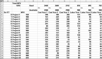
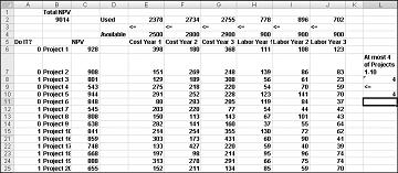
Most corporations want to undertake projects that contribute the greatest net present value (NPV), subject to limited resources (usually capital and labor). Let’s say that a software development company is trying to determine which of 20 software projects it should undertake. The NPV (in millions of dollars) contributed by each project as well as the capital (in millions of dollars) and the number of programmers needed during each of the next three years is given on the Basic Model worksheet in the file Capbudget.xlsx, which is shown in Figure 30-1 on the next page. For example, Project 2 yields $908 million. It requires $151 million during Year 1, $269 million during Year 2, and $248 million during Year 3. Project 2 requires 139 programmers during Year 1, 86 programmers during Year 2, and 83 programmers during Year 3. Cells E4:G4 show the capital (in millions of dollars) available during each of the three years, and cells H4:J4 indicate how many programmers are available. For example, during Year 1 up to $2.5 billion in capital and 900 programmers are available.
The company must decide whether it should undertake each project. Let’s assume that we can’t undertake a fraction of a software project; if we allocate 0.5 of the needed resources, for example, we would have a nonworking program that would bring us $0 revenue!
The trick in modeling situations in which you either do or don’t do something is to use binary changing cells. A binary changing cell always equals 0 or 1. When a binary changing cell that corresponds to a project equals 1, we do the project. If a binary changing cell that corresponds to a project equals 0, we don’t do the project. You set up Solver to use a range of binary changing cells by adding a constraint—select the changing cells you want to use and then choose Bin from the list in the Add Constraint dialog box.
With this background, we’re ready to solve the software project selection problem. As always with a Solver model, we begin by identifying our target cell, the changing cells, and the constraints.
-
Target cell. We maximize the NPV generated by selected projects.
-
Changing cells. We look for a 0 or 1 binary changing cell for each project. I’ve located these cells in the range A6:A25 (and named the range doit). For example, a 1 in cell A6 indicates that we undertake Project 1; a 0 in cell C6 indicates that we don’t undertake Project 1.
-
Constraints. We need to ensure that for each Year t (t=1, 2, 3), Year t capital used is less than or equal to Year t capital available, and Year t labor used is less than or equal to Year t labor available.
As you can see, our worksheet must compute for any selection of projects the NPV, the capital used annually, and the programmers used each year. In cell B2, I use the formula SUMPRODUCT(doit,NPV) to compute the total NPV generated by selected projects. (The range name NPV refers to the range C6:C25.) For every project with a 1 in column A, this formula picks up the NPV of the project, and for every project with a 0 in column A, this formula does not pick up the NPV of the project. Therefore, we’re able to compute the NPV of all projects, and our target cell is linear because it is computed by summing terms that follow the form (changing cell)*(constant). In a similar fashion, I compute the capital used each year and the labor used each year by copying from E2 to F2:J2 the formula SUMPRODUCT(doit,E6:E25).
I now fill in the Solver Parameters dialog box as shown in Figure 30-2.
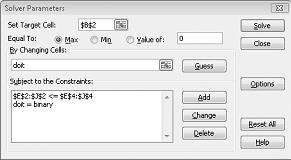
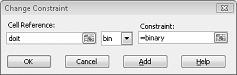
Our goal is to maximize NPV of selected projects (cell B2). Our changing cells (the range named doit) are the binary changing cells for each project. The constraint E2:J2<=E4:J4 ensures that during each year the capital and labor used are less than or equal to the capital and labor available. To add the constraint that makes the changing cells binary, I click Add in the Solver Parameters dialog box and then select Bin from the list in the middle of the dialog box. The Add Constraint dialog box should appear as shown in Figure 30-3.
Our model is linear because the target cell is computed as the sum of terms that have the form (changing cell)*(constant) and because the resource usage constraints are computed by comparing the sum of (changing cells)*(constants) to a constant.
With the Solver Parameters dialog box filled in, click Solve and we have the results shown earlier in Figure 30-1. The company can obtain a maximum NPV of $9,293 million ($9.293 billion) by choosing Projects 2, 3, 6–10, 14–16, 19, and 20.
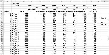
Sometimes project-selection models have other constraints. For example, suppose that if we select Project 3, we must also select Project 4. Because our current optimal solution selects Project 3 but not Project 4, we know that our current solution can’t remain optimal. To solve this problem, simply add the constraint that the binary changing cell for Project 3 is less than or equal to the binary changing cell for Project 4.
You can find this example on the If 3 then 4 worksheet in the file Capbudget.xlsx, which is shown in Figure 30-4. Cell L9 refers to the binary value related to Project 3, and cell L12 to the binary value related to Project 4. By adding the constraint L9<=L12, if we choose Project 3, L9 equals 1 and our constraint forces L12 (the Project 4 binary) to equal 1. Our constraint must also leave the binary value in the changing cell of Project 4 unrestricted if we do not select Project 3. If we do not select Project 3, L9 equals 0 and our constraint allows the Project 4 binary to equal 0 or 1, which is what we want. The new optimal solution is shown in Figure 30-4.
A new optimal solution is calculated if selecting Project 3 means we must also select Project 4. Now suppose that we can do only four projects from among Projects 1 through 10. (See the At Most 4 Of P1–P10 worksheet, shown in Figure 30-5.) In cell L8, we compute the sum of the binary values associated with Projects 1 through 10 with the formula SUM(A6:A15). Then we add the constraint L8<=L10, which ensures that, at most, 4 of the first 10 projects are selected. The new optimal solution is shown in Figure 30-5. The NPV has dropped to $9.014 billion.
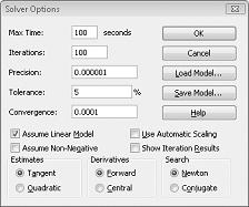
Linear Solver models in which some or all changing cells are required to be binary or integer are usually harder to solve than linear models in which all changing cells are allowed to be fractions. For this reason, we often are satisfied with a near-optimal solution to a binary or integer programming problem. If your Solver model runs for a long time, you may want to consider adjusting the Tolerance setting in the Solver Options dialog box. (See Figure 30-6.) For example, a Tolerance setting of 0.5% means that Solver will stop the first time it finds a feasible solution that is within 0.5 percent of the theoretical optimal target cell value (the theoretical optimal target cell value is the optimal target value found when the binary and integer constraints are omitted). Often we are faced with a choice between finding an answer within 10 percent of optimal in 10 minutes or finding an optimal solution in two weeks of computer time! The default Tolerance value is 0.05%, which means that Solver stops when it finds a Target cell value within 0.05 percent of the theoretical optimal target cell value.
-
A company has nine projects under consideration. The NPV added by each project and the capital required by each project during the next two years is shown in the following table. (All numbers are in millions.) For example, Project 1 will add $14 million in NPV and require expenditures of $12 million during Year 1 and $3 million during Year 2. During Year 1, $50 million in capital is available for projects, and $20 million is available during Year 2.
|
NPV |
Year 1 expenditure |
Year 2 expenditure |
|
|---|---|---|---|
|
Project 1 |
14 |
12 |
3 |
|
Project 2 |
17 |
54 |
7 |
|
Project 3 |
17 |
6 |
6 |
|
Project 4 |
15 |
6 |
2 |
|
Project 5 |
40 |
30 |
35 |
|
Project 6 |
12 |
6 |
6 |
|
Project 7 |
14 |
48 |
4 |
|
Project 8 |
10 |
36 |
3 |
|
Project 9 |
12 |
18 |
3 |
-
If we can’t undertake a fraction of a project but must undertake either all or none of a project, how can we maximize NPV?
-
Suppose that if Project 4 is undertaken, Project 5 must be undertaken. How can we maximize NPV?
-
A publishing company is trying to determine which of 36 books it should publish this year. The file Pressdata.xlsx gives the following information about each book:
-
Projected revenue and development costs (in thousands of dollars)
-
Pages in each book
-
Whether the book is geared toward an audience of software developers (indicated by a 1 in column E)
A publishing company can publish books totaling up to 8500 pages this year and must publish at least four books geared toward software developers. How can the company maximize its profit?
-
This article was adapted from Microsoft Office Excel 2007 Data Analysis and Business Modeling by Wayne L. Winston.
This classroom-style book was developed from a series of presentations by Wayne Winston, a well known statistician and business professor who specializes in creative, practical applications of Excel.


