
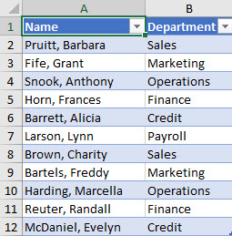
Sorting data is an integral part of data analysis. You might want to arrange a list of names in alphabetical order, compile a list of product inventory levels from highest to lowest, or order rows by colors or icons. Sorting data helps you quickly visualize and understand your data better, organize and find the data that you want, and ultimately make more effective decisions.
You can sort data by text (A to Z or Z to A), numbers (smallest to largest or largest to smallest), and dates and times (oldest to newest and newest to oldest) in one or more columns. You can also sort by a custom list you create (such as Large, Medium, and Small) or by format, including cell color, font color, or icon set. To find the top or bottom values in a range of cells or table, such as the top 10 grades or the bottom 5 sales amounts, use AutoFilter or conditional formatting. Check out the video to see how it's done.
-
Select a cell in the column you want to sort.
-
On the Data tab, in the Sort & Filter group, do one of the following:
-
To quick sort in ascending order, click

-
To quick sort in descending order, click

-
Notes: Potential Issues
-
Check that all data is stored as text If the column that you want to sort contains numbers stored as numbers and numbers stored as text, you need to format them all as either numbers or text. If you do not apply this format, the numbers stored as numbers are sorted before the numbers stored as text. To format all the selected data as text, Press Ctrl+1 to launch the Format Cells dialog, click the Number tab and then, under Category, click General, Number, or Text.
-
Remove any leading spaces In some cases, data imported from another application might have leading spaces inserted before data. Remove the leading spaces before you sort the data. You can do this manually, or you can use the TRIM function.
-
Select a cell in the column you want to sort.
-
On the Data tab, in the Sort & Filter group, do one of the following:
-
To sort from low to high, click
-
To sort from high to low, click
-
Notes:
-
Potential Issue
-
Check that all numbers are stored as numbers If the results are not what you expected, the column might contain numbers stored as text instead of as numbers. For example, negative numbers imported from some accounting systems, or a number entered with a leading apostrophe (') are stored as text. For more information, see Fix text-formatted numbers by applying a number format.
-
Select a cell in the column you want to sort.
-
On the Data tab, in the Sort & Filter group, do one of the following:
-
To sort from an earlier to a later date or time, click
-
To sort from a later to an earlier date or time, click
-
Notes: Potential Issue
-
Check that dates and times are stored as dates or times If the results are not what you expected, the column might contain dates or times stored as text instead of as dates or times. For Excel to sort dates and times correctly, all dates and times in a column must be stored as a date or time serial number. If Excel cannot recognize a value as a date or time, the date or time is stored as text. For more information, see Convert dates stored as text to dates.
-
If you want to sort by days of the week, format the cells to show the day of the week. If you want to sort by the day of the week regardless of the date, convert them to text by using the TEXT function. However, the TEXT function returns a text value, so the sort operation would be based on alphanumeric data. For more information, see Show dates as days of the week.
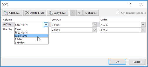
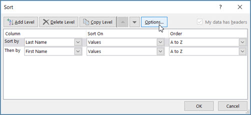
You may want to sort by more than one column or row when you have data that you want to group by the same value in one column or row, and then sort another column or row within that group of equal values. For example, if you have a Department column and an Employee column, you can first sort by Department (to group all the employees in the same department together), and then sort by name (to put the names in alphabetical order within each department). You can sort by up to 64 columns.
Note: For best results, the range of cells that you sort should have column headings.
-
Select any cell in the data range.
-
On the Data tab, in the Sort & Filter group, click Sort.

-
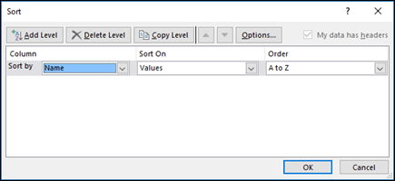
In the Sort dialog box, under Column, in the Sort by box, select the first column that you want to sort.
-
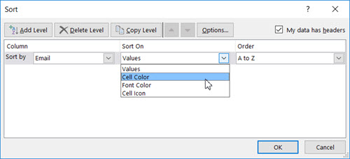
Under Sort On, select the type of sort. Do one of the following:
-
To sort by text, number, or date and time, select Values.
-
To sort by format, select Cell Color, Font Color, or Cell Icon.
-
-
Under Order, select how you want to sort. Do one of the following:
-
For text values, select A to Z or Z to A.
-
For number values, select Smallest to Largest or Largest to Smallest.
-
For date or time values, select Oldest to Newest or Newest to Oldest.
-
To sort based on a custom list, select Custom List.
-
-
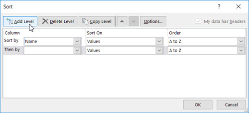
To add another column to sort by, click Add Level, and then repeat steps three through five.
-
To copy a column to sort by, select the entry and then click Copy Level.
-
To delete a column to sort by, select the entry and then click Delete Level.
Note: You must keep at least one entry in the list.
-
To change the order in which the columns are sorted, select an entry and then click the Up or Down arrow next to the Options button to change the order.
Entries higher in the list are sorted before entries lower in the list.
If you have manually or conditionally formatted a range of cells or a table column by cell color or font color, you can also sort by these colors. You can also sort by an icon set that you created with conditional formatting.
-
Select a cell in the column you want to sort.
-
On the Data tab, in the Sort & Filter group, click Sort.
-
In the Sort dialog box, under Column, in the Sort by box, select the column that you want to sort.
-
Under Sort On, select Cell Color, Font Color, or Cell Icon.
-
Under Order, click the arrow next to the button and then, depending on the type of format, select a cell color, font color, or cell icon.
-
Next, select how you want to sort. Do one of the following:
-
To move the cell color, font color, or icon to the top or to the left, select On Top for a column sort, and On Left for a row sort.
-
To move the cell color, font color, or icon to the bottom or to the right, select On Bottom for a column sort, and On Right for a row sort.
Note: There is no default cell color, font color, or icon sort order. You must define the order that you want for each sort operation.
-
-
To specify the next cell color, font color, or icon to sort by, click Add Level, and then repeat steps three through five.
Make sure that you select the same column in the Then by box and that you make the same selection under Order.
Keep repeating for each additional cell color, font color, or icon that you want included in the sort.
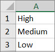
You can use a custom list to sort in a user-defined order. For example, a column might contain values that you want to sort by, such as High, Medium, and Low. How can you sort so that rows containing High appear first, followed by Medium, and then Low? If you were to sort alphabetically, an “A to Z” sort would put High at the top, but Low would come before Medium. And if you sorted “Z to A,” Medium would appear first, with Low in the middle. Regardless of the order, you always want “Medium” in the middle. By creating your own custom list, you can get around this problem.
-
Optionally, create a custom list:
-
In a range of cells, enter the values that you want to sort by, in the order that you want them, from top to bottom as in this example.
-
Select the range that you just entered. Using the preceding example, select cells A1:A3.
-
Go to File > Options > Advanced > General > Edit Custom Lists, then in the Custom Lists dialog box, click Import, and then click OK twice.
Notes:
-
You can create a custom list based only on a value (text, number, and date or time). You cannot create a custom list based on a format (cell color, font color, or icon).
-
The maximum length for a custom list is 255 characters, and the first character must not begin with a number.
-
-
-
Select a cell in the column you want to sort.
-
On the Data tab, in the Sort & Filter group, click Sort.
-
In the Sort dialog box, under Column, in the Sort by or Then by box, select the column that you want to sort by a custom list.
-
Under Order, select Custom List.
-
In the Custom Lists dialog box, select the list that you want. Using the custom list that you created in the preceding example, click High, Medium, Low.
-
Click OK.
-
On the Data tab, in the Sort & Filter group, click Sort.
-
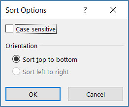
In the Sort dialog box, click Options.
-
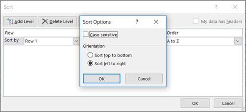
In the Sort Options dialog box, select Case sensitive.
-
Click OK twice.
It's most common to sort from top to bottom, but you can also sort from left to right.
Note: Tables don't support left to right sorting. To do so, first convert the table to a range by selecting any cell in the table, and then clicking Table Tools > Convert to range.
-
Select any cell within the range you want to sort.
-
On the Data tab, in the Sort & Filter group, click Sort.
-
In the Sort dialog box, click Options.
-
In the Sort Options dialog box, under Orientation, click Sort left to right, and then click OK.
-
Under Row, in the Sort by box, select the row that you want to sort. This will generally be row 1 if you want to sort by your header row.
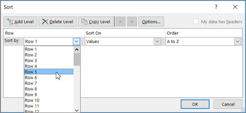
Tip: If your header row is text, but you want to order columns by numbers, you can add a new row above your data range and add numbers according to the order you want them.
-
To sort by value, select one of the options from the Order drop-down:
-
For text values, select A to Z or Z to A.
-
For number values, select Smallest to Largest or Largest to Smallest.
-
For date or time values, select Oldest to Newest or Newest to Oldest.
-
-
To sort by cell color, font color, or cell icon, do this:
-
Under Sort On, select Cell Color, Font Color, or Cell Icon.
-
Under Order select a cell color, font color, or cell icon, then select On Left or On Right.
-
Note: When you sort rows that are part of a worksheet outline, Excel sorts the highest-level groups (level 1) so that the detail rows or columns stay together, even if the detail rows or columns are hidden.
To sort by a part of a value in a column, such as a part number code (789-WDG-34), last name (Carol Philips), or first name (Philips, Carol), you first need to split the column into two or more columns so that the value you want to sort by is in its own column. To do this, you can use text functions to separate the parts of the cells or you can use the Convert Text to Columns Wizard. For examples and more information, see Split text into different cells and Split text among columns by using functions.
Warning: It is possible to sort a range within a range, but it is not recommended, because the result disassociates the sorted range from its original data. If you were to sort the following data as shown, the selected employees would be associated with different departments than they were before.
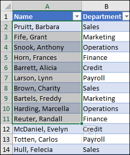
Fortunately, Excel will warn you if it senses you are about to attempt this:

If you did not intend to sort like this, then press the Expand the selection option, otherwise select Continue with the current selection.
If the results are not what you want, click Undo 
Note: You cannot sort this way in a table.
If you get unexpected results when sorting your data, do the following:
Check to see if the values returned by a formula have changed If the data that you have sorted contains one or more formulas, the return values of those formulas might change when the worksheet is recalculated. In this case, make sure that you reapply the sort to get up-to-date results.
Unhide rows and columns before you sort Hidden columns are not moved when you sort columns, and hidden rows are not moved when you sort rows. Before you sort data, it's a good idea to unhide the hidden columns and rows.
Check the locale setting Sort orders vary by locale setting. Make sure that you have the proper locale setting in Regional Settings or Regional and Language Options in Control Panel on your computer. For information about changing the locale setting, see the Windows help system.
Enter column headings in only one row If you need multiple line labels, wrap the text within the cell.
Turn on or off the heading row It's usually best to have a heading row when you sort a column to make it easier to understand the meaning of the data. By default, the value in the heading is not included in the sort operation. Occasionally, you may need to turn the heading on or off so that the value in the heading is or is not included in the sort operation. Do one of the following:
-
To exclude the first row of data from the sort because it is a column heading, on the Home tab, in the Editing group, click Sort & Filter, click Custom Sort and then select My data has headers.
-
To include the first row of data in the sort because it is not a column heading, on the Home tab, in the Editing group, click Sort & Filter, click Custom Sort, and then clear My data has headers.
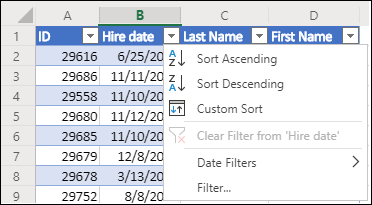
If your data is formatted as an Excel table, then you can quickly sort and filter it with the filter buttons in the header row.
-
If your data isn't already in a table, then format it as a table. This will automatically add a filter button at the top of each table column.
-
Click the filter button at the top of the column you want to sort on, and pick the sort order you want.
-
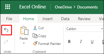
To undo a sort, use the Undo button on the Home tab.
-
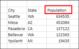
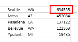
Pick a cell to sort on:
-
If your data has a header row, pick the one you want to sort on, such as Population.
-
If your data doesn’t have a header row, pick the topmost value you want to sort on, such as 634535.
-
-
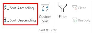
On the Data tab, pick one of the sort methods:
-
Sort Ascending to sort A to Z, smallest to largest, or earliest to latest date.
-
Sort Descending to sort Z to A, largest to smallest, or latest to earliest date.
-
Let's say you have a table with a Department column and an Employee column. You can first sort by Department to group all the employees in the same department together, and then sort by name to put the names in alphabetical order within each department.
Select any cell within your data range.
-
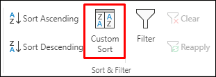
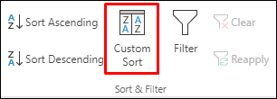
On the Data tab, in the Sort & Filter group, click Custom Sort.
-
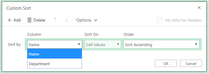
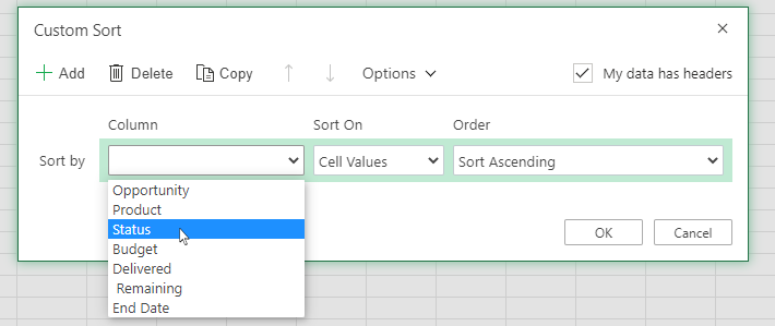
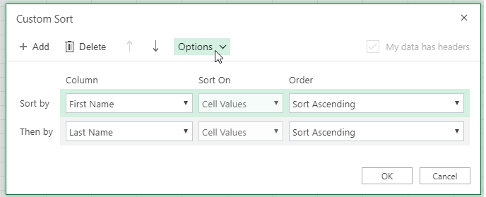
In the Custom Sort dialog box, under Column, in the Sort by box, select the first column that you want to sort.
Note: The Sort On menu is disabled because it's not yet supported. For now, you can change it in the Excel desktop app.
-
Under Order, select how you want to sort:
-
Sort Ascending to sort A to Z, smallest to largest, or earliest to latest date.
-
Sort Descending to sort Z to A, largest to smallest, or latest to earliest date.
-
-
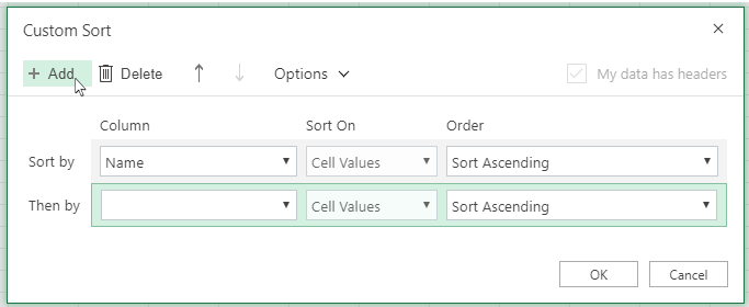
To add another column to sort by, click Add and then repeat steps five and six.
-
To change the order in which the columns are sorted, select an entry and then click the Up or Down arrow next to the Options button.
If you have manually or conditionally formatted a range of cells or a table column by cell color or font color, you can also sort by these colors. You can also sort by an icon set that you created with conditional formatting.
-
Select a cell in the column you want to sort
-
On the Data tab, in the Sort & Filter group, select Custom Sort.
-
In the Custom Sort dialog box under Columns, select the column that you want to sort.
-
Under Sort On, select Cell Color, Font Color or Conditional Formatting Icon.
-
Under Order, select the order you want (what you see depends on the type of format you have). Then select a cell color, font color, or cell icon.
-
Next, you'll choose how you want to sort by moving the cell color, font color, or icon:
Note: There is no default cell color, font color, or icon sort order. You must define the order that you want for each sort operation.
-
To move to the top or to the left: Select On Top for a column sort, and On Left for a row sort.
-
To move to the bottom or to the right: Select On Bottom for a column sort, and On Right for a row sort.
-
-
To specify the next cell color, font color, or icon to sort by, select Add Level, and then repeat steps 1- 5.
-
Make sure that you the column in the Then by box and the selection under Order are the same.
-
Repeat for each additional cell color, font color, or icon that you want included in the sort.
-
On the Data tab, in the Sort & Filter group, click Custom Sort.
-
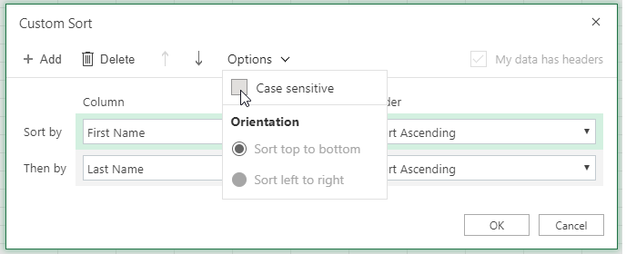
In the Custom Sort dialog box, click Options.
-
In the Options menu, select Case sensitive.
-
Click OK.
It's most common to sort from top to bottom, but you can also sort from left to right.
Note: Tables don't support left to right sorting. To do so, first convert the table to a range by selecting any cell in the table, and then clicking Table Tools > Convert to range.
-
Select any cell within the range you want to sort.
-
On the Data tab, in the Sort & Filter group, select Custom Sort.
-
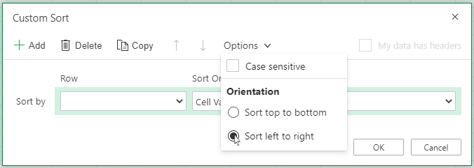
In the Custom Sort dialog box, click Options.
-
Under Orientation, click Sort left to right
-
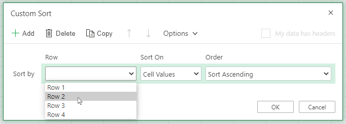
Under Row, in the 'Sort by' drop down, select the row that you want to sort. This will generally be row 1 if you want to sort by your header row.
-
To sort by value, select one of the options from the Order drop-down:
-
Sort Ascending to sort A to Z, smallest to largest, or earliest to latest date.
-
Sort Descending to sort Z to A, largest to smallest, or latest to earliest date
-
See how it's done

Need more help?
You can always ask an expert in the Excel Tech Community or get support in Communities.
See also
Use the SORT and SORTBY functions to automatically sort your data. Also, see Filter data in an Excel table or range, and Apply conditional formatting in Excel.


