
If Excel can’t resolve a formula you’re trying to create, you may get an error message like this one:
Unfortunately, this means that Excel can’t understand what you’re trying to do, so you'll need to update your formula or make sure you're using the function correctly.
Tip: There are a few common functions where you might run into issues. To learn more, check out COUNTIF, SUMIF, VLOOKUP, or IF. You can also see a list of functions here.
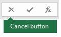
Return to the cell with the broken formula, which will be in edit mode, and Excel will highlight the spot where it’s having a problem. If you still don’t know what to do from there and want to start over, you can press ESC again, or select the Cancel button in the formula bar, which will take you out of edit mode.
If you want to move forward, then the following checklist provides troubleshooting steps to help you figure out what may have gone wrong. Select the headings to learn more.
Note: If you're using Microsoft 365 for the web, you may not see the same errors, or the solutions may not apply.
Formulas with more than one argument use list separators to separate their arguments. Which separator is used can vary based on your OS Locale and Excel settings. The most common list separators are comma "," and semicolon ";".
A formula will break if any of its functions use incorrect delimiters.
For more information, please see: Formula errors when list separator is not set correctly
Excel throws a variety of pound (#) errors such as #VALUE!, #REF!, #NUM, #N/A, #DIV/0!, #NAME?, and #NULL!, to indicate something in your formula isn't working properly. For example, the #VALUE! error is caused by incorrect formatting or unsupported data types in arguments. Or, you'll see the #REF! error if a formula refers to cells that have been deleted or replaced with other data. Troubleshooting guidance will differ for each error.
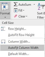
Note: #### is not a formula-related error. It just means that the column isn't wide enough to display the cell contents. Simply drag the column to widen it, or go to Home > Format > AutoFit Column Width.
Refer to any of the following topics corresponding to the pound error you see:
Each time you open a spreadsheet that contains formulas referring to values in other spreadsheets, you'll be prompted to update the references or leave them as-is.
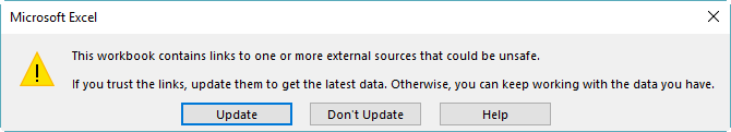
Excel displays the above dialog box to make sure that the formulas in the current spreadsheet always point to the most updated value in case the reference value has changed. You can choose to update the references, or skip if you don't want to update. Even if you choose to not update the references, you can always manually update the links in the spreadsheet whenever you want.
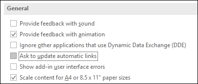
You can always disable the dialog box from appearing at start up. To do that, go to File > Options > Advanced > General, and clear the Ask to update automatic links box.
Important: If this is the first time you're working with broken links in formulas, if you need a refresher on resolving broken links, or if you don't know whether to update the references, see Control when external references (links) are updated.
If the formula doesn't display the value, follow these steps:
-
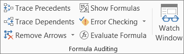
Make sure Excel is set to show formulas in your spreadsheet. To do this, select the Formulas tab, and in the Formula Auditing group, select Show Formulas.
Tip: You can also use the keyboard shortcut Ctrl + ` (the key above the Tab key). When you do this, your columns will automatically widen to display your formulas, but don’t worry, when you toggle back to the normal view, your columns will resize.
-
If the step above still doesn't resolve the issue, it's possible the cell is formatted as text. You can right-click on the cell and select Format Cells > General (or Ctrl + 1), then press F2 > Enter to change the format.
-
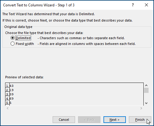
If you have a column with a large range of cells that are formatted as text, you can select the range, apply the number format of your choice, and go to Data > Text to Column > Finish. This will apply the format to all of the selected cells.
When a formula does not calculate, you'll need to check if automatic calculation is enabled in Excel. Formulas won't calculate if manual calculation is enabled. Follow these steps to check for Automatic calculation.
-
Select the File tab, select Options, and then select the Formulas category.
-
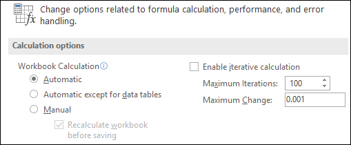
In the Calculation options section, under Workbook Calculation, make sure the Automatic option is selected.
For more information on calculations, see Change formula recalculation, iteration, or precision.
A circular reference occurs when a formula refers to the cell that it's located in. The fix is to either move the formula to another cell, or change the formula syntax to one that avoids circular references. However, in some scenarios you may need circular references because they cause your functions to iterate—repeat until a specific numeric condition is met. In such cases, you'll need to enable Remove or allow a circular reference.
For more information on circular references, see Remove or allow a circular reference.
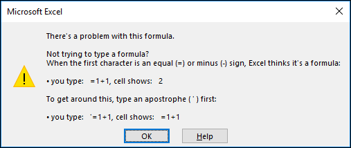
If your entry doesn’t start with an equal sign, it isn’t a formula, and won’t be calculated—a common mistake.
When you type something like SUM(A1:A10), Excel shows the text string SUM(A1:A10) instead of a formula result. Alternatively, if you type 11/2, Excel shows a date, such as 2-Nov or 11/02/2009, instead of dividing 11 by 2.
To avoid these unexpected results, always start the function with an equal sign. For example, type: =SUM(A1:A10) and =11/2.
When you use a function in a formula, each opening parenthesis needs a closing parenthesis for the function to work correctly. Make sure that all parentheses are part of a matching pair. For example, the formula =IF(B5<0),"Not valid",B5*1.05) won’t work because there are two closing parentheses, but only one opening parenthesis. The correct formula would look like this: =IF(B5<0,"Not valid",B5*1.05).
Excel functions have arguments—values you need to provide for the function to work. Only a few functions (such as PI or TODAY) take no arguments. Check the formula syntax that appears as you start typing in the function, to make sure the function has the required arguments.
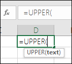
For example, the UPPER function accepts only one string of text or cell reference as its argument: =UPPER("hello") or =UPPER(C2)
Note: You'll see the function’s arguments listed in a floating function reference toolbar beneath the formula as you're typing it.
Also, some functions, such as SUM, require numerical arguments only, while other functions, such as REPLACE, require a text value for at least one of their arguments. If you use the wrong data type, functions might return unexpected results or show a #VALUE! error.
If you need to quickly look up the syntax of a particular function, see the list of Excel functions (by category).
Don't enter numbers formatted with dollar signs ($) or decimal separators (,) in formulas because dollar signs indicate Absolute References and commas are argument separators. Instead of entering $1,000, enter 1000 in the formula.
If you use formatted numbers in arguments, you’ll get unexpected calculation results, but you may also see the #NUM! error. For example, if you enter the formula =ABS(-2,134) to find the absolute value of -2134, Excel shows the #NUM! error, because the ABS function accepts only one argument, and it sees the -2, and 134 as separate arguments.
Note: You can format the formula result with decimal separators and currency symbols after you enter the formula using unformatted numbers (constants). It’s generally not a good idea to put constants in formulas, because they can be hard to find if you need to update later and they're more prone to being typed incorrectly. It’s much better to put your constants in cells, where they're out in the open and easily referenced.
Your formula might not return expected results if the cell’s data type can’t be used in calculations. For example, if you enter a simple formula =2+3 in a cell that’s formatted as text, Excel can’t calculate the data you entered. All you'll see in the cell is =2+3. To fix this, change the cell’s data type from Text to General like this:
-
Select the cell.
-
Select Home and select the arrow to expand the Number or Number Format group (or press Ctrl + 1). Then select General.
-
Press F2 to put the cell in the edit mode, and then press Enter to accept the formula.
A date you enter in a cell that’s using the Number data type might be shown as a numeric date value instead of a date. To show a number as a date, pick a Date format in the Number Format gallery.
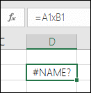
It's fairly common to use x as the multiplication operator in a formula, but Excel can only accept the asterisk (*) for multiplication. If you use constants in your formula, Excel shows an error message and can fix the formula for you by replacing the x with the asterisk (*).
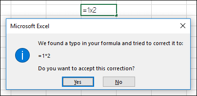
However, if you use cell references, Excel will return a #NAME? error.
If you create a formula that includes text, enclose the text in quotation marks.
For example, the formula ="Today is " & TEXT(TODAY(),"dddd, mmmm dd") combines the text "Today is " with the results of the TEXT and TODAY functions, and returns say something like Today is Monday, May 30.
In the formula, "Today is " has a space before the ending quotation mark to provide the blank space you want between the words "Today is" and "Monday, May 30." Without quotation marks around the text, the formula might show the #NAME? error.
You can combine (or nest) up to 64 levels of functions within a formula.
For example, the formula =IF(SQRT(PI())<2,"Less than two!","More than two!") has 3 levels of functions; the PI function is nested inside the SQRT function, which in turn is nested inside the IF function.
When you type a reference to values or cells in another worksheet, and the name of that sheet has a non-alphabetical character (such as a space), enclose the name in single quotation marks (').
For example, to return the value from cell D3 in a worksheet named Quarterly Data in your workbook, type: ='Quarterly Data'!D3. Without the quotation marks around the sheet name, the formula shows the #NAME? error.
You can also select the values or cells in another sheet to refer to them in your formula. Excel then automatically adds the quotation marks around the sheet names.
When you type a reference to values or cells in another workbook, include the workbook name enclosed in square brackets ([]) followed by the name of the worksheet that has the values or cells.
For example, to refer to cells A1 through A8 on the Sales sheet in the Q2 Operations workbook that’s open in Excel, type: =[Q2 Operations.xlsx]Sales!A1:A8. Without the square brackets, the formula shows the #REF! error.
If the workbook isn’t open in Excel, type the full path to the file.
For example, =ROWS('C:\My Documents\[Q2 Operations.xlsx]Sales'!A1:A8).
Note: If the full path has space characters, enclose the path in single quotation marks (at the beginning of the path and after the name of the worksheet, before the exclamation point).
Tip: The easiest way to get the path to the other workbook is to open the other workbook, then from your original workbook, type =, and use Alt+Tab to shift to the other workbook. Select any cell on the sheet you want, then close the source workbook. Your formula will automatically update to display the full file path and sheet name along with the required syntax. You can even copy and paste the path and use wherever you need it.
Dividing a cell by another cell that has zero (0) or no value results in a #DIV/0! error.
To avoid this error, you can address it directly and test for the existence of the denominator. You could use:
=IF(B1,A1/B1,0)
Which says IF(B1 exists, then divide A1 by B1, otherwise return a 0).
Always check to see if you have any formulas that refer to data in cells, ranges, defined names, worksheets, or workbooks before you delete anything. You can then replace these formulas with their results before you remove the referenced data.
If you can’t replace the formulas with their results, review this information about the errors and possible solutions:
-
If a formula refers to cells that have been deleted or replaced with other data, and if it returns a #REF! error, select the cell with the #REF! error. In the formula bar, select #REF! and delete it. Then enter the range for the formula again.
-
If a defined name is missing, and a formula that refers to that name returns a #NAME? error, define a new name that refers to the range you want, or change the formula to refer directly to the range of cells (for example, A2:D8).
-
If a worksheet is missing, and a formula that refers to it returns a #REF! error, there’s no way to fix this, unfortunately—a worksheet that’s been deleted can't be recovered.
-
If a workbook is missing, a formula that refers to it remains intact until you update the formula.
For example, if your formula is =[Book1.xlsx]Sheet1'!A1 and you no longer have Book1.xlsx, the values referenced in that workbook stay available. However, if you edit and save a formula that refers to that workbook, Excel shows the Update Values dialog box and prompts you to enter a file name. Select Cancel, and then make sure this data isn’t lost by replacing the formulas that refer to the missing workbook with the formula results.
Sometimes, when you copy the contents of a cell, you want to paste just the value and not the underlying formula that's displayed in the formula bar.
For example, you might want to copy the resulting value of a formula to a cell on another worksheet. Or you might want to delete the values that you used in a formula after you copied the resulting value to another cell on the worksheet. Both of these actions cause an invalid cell reference error (#REF!) to appear in the destination cell, because the cells that contain the values you used in the formula can no longer be referenced.
You can avoid this error by pasting the resulting values of formulas, without the formula, in destination cells.
-
On a worksheet, select the cells that contain the resulting values of a formula that you want to copy.
-
On the Home tab, in the Clipboard group, select Copy

Keyboard shortcut: Press CTRL+C.
-
Select the upper-left cell of the paste area.
Tip: To move or copy a selection to a different worksheet or workbook, select another worksheet tab or switch to another workbook, and then select the upper-left cell of the paste area.
-
On the Home tab, in the Clipboard group, select Paste

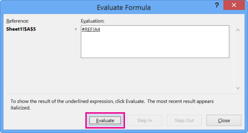
To understand how a complex or nested formula calculates the final result, you can evaluate that formula.
-
Select the formula you want to evaluate.
-
Select Formulas > Evaluate Formula.
-
Select Evaluate to examine the value of the underlined reference. The result of the evaluation is shown in italics.
-
If the underlined part of the formula is a reference to another formula, select Step In to show the other formula in the Evaluation box. Select Step Out to go back to the previous cell and formula.
The Step In button isn’t available the second time the reference appears in the formula—or if the formula refers to a cell in another workbook.
-
Continue until each part of the formula has been evaluated.
The Evaluate Formula tool won't necessarily tell you why your formula is broken, but it can help point out where. This can be a very handy tool in larger formulas where it might otherwise be difficult to find the problem.
Notes:
-
Some parts of the IF and CHOOSE functions won’t be evaluated, and the #N/A error might appear in the Evaluation box.
-
Blank references are shown as zero values (0) in the Evaluation box.
-
Some functions are recalculated every time the worksheet changes. Those functions, including the RAND, AREAS, INDEX, OFFSET, CELL, INDIRECT, ROWS, COLUMNS, NOW, TODAY, and RANDBETWEEN functions, can cause the Evaluate Formula dialog box to show results that are different from the actual results in the cell on the worksheet.
-
Need more help?
You can always ask an expert in the Excel Tech Community or get support in Communities.
Tip: If you're a small business owner looking for more information on how to get Microsoft 365 set up, visit Small business help & learning.


